Benchmark della proiezione degli operatori di Pauli

Azione di una stringa di Pauli su uno stato della base computazionale

L'azione di una stringa di Pauli su uno stato della base computazionale è piuttosto banale ed è essa stessa un singolo stato della base computazionale. Ciò è una conseguenza diretta della struttura delle matrici di Pauli, che hanno un solo elemento non nullo su ciascuna riga. Di conseguenza, la loro azione su un qubit è:

---

$$\sigma_x |0 \rangle = |1 \rangle$$ $$\sigma_x |1 \rangle = |0 \rangle$$

---

$$\sigma_y |0 \rangle = i|1 \rangle$$ $$\sigma_y |1 \rangle = -i|0 \rangle$$

---

$$\sigma_z |0 \rangle = |0 \rangle$$ $$\sigma_z |1 \rangle = -|1 \rangle$$

---

$$I |0 \rangle = |0 \rangle$$ $$I |1 \rangle = |1 \rangle$$

---

Ogni bit della bitstring che etichetta la base computazionale sarà indicato con $x \in \{0, 1 \}$. Per mantenere l'implementazione il più leggera possibile, rappresenteremo le bitstring con variabili bool: $0\rightarrow \textrm{False}$ e $1\rightarrow \textrm{True}$.

Per rappresentare l'azione di ciascun operatore di Pauli su uno stato della base computazionale, glie assegneremo tre variabili: diag, sign, imag.

• diag indica se l'operatore è diagonale:

  • $\textrm{diag}(I) = \textrm{True}$

  • $\textrm{diag}(\sigma_x) = \textrm{False}$

  • $\textrm{diag}(\sigma_y) = \textrm{False}$

  • $\textrm{diag}(\sigma_z) = \textrm{True}$

• sign identifica se c'è un cambio di segno nell'elemento di matrice collegato a 0 oppure a 1:

  • $\textrm{sign}(I) = \textrm{False}$

  • $\textrm{sign}(\sigma_x) = \textrm{False}$

  • $\textrm{sign}(\sigma_y) = \textrm{True}$

  • $\textrm{sign}(\sigma_z) = \textrm{True}$

• imag identifica se l'elemento di matrice ha una componente complessa:

  • $\textrm{imag}(I) = \textrm{False}$

  • $\textrm{imag}(\sigma_x) = \textrm{False}$

  • $\textrm{imag}(\sigma_y) = \textrm{True}$

  • $\textrm{imag}(\sigma_z) = \textrm{False}$

Indichiamo un operatore di Pauli arbitrario con $\sigma \in \{ I, \sigma_x, \sigma_y \sigma_z\}$. L'azione dell'operatore di Pauli su uno stato della base computazionale può quindi essere rappresentata dall'operazione logica:

$$\sigma |x \rangle = |x == \textrm{diag}(\sigma) \rangle (-1)^{x\textrm{ and sign}(\sigma)} (i)^{\textrm{imag}(\sigma)}.$$

Lo stesso si generalizza direttamente a un numero arbitrario di qubit. Verifichiamo che funzioni:

# Added by doQumentation — installs the packages this notebook needs if they are missing
import importlib.util

_needed = {"matplotlib": "matplotlib", "numpy": "numpy", "qiskit": "qiskit", "qiskit_addon_sqd": "qiskit-addon-sqd"}
_missing = [pip for module, pip in _needed.items()
            if importlib.util.find_spec(module) is None]
# One at a time, so a package that fails to install does not block the others
for _pip in _missing:
    %pip install -q {_pip}
if not _missing:
    print("\u2713 All required packages are installed")

def connected_element_and_amplitude_bool(
    x: bool, diag: bool, sign: bool, imag: bool
) -> tuple[bool, complex]:
    """
    Finds the connected element to computational basis state |x> under
    the action of the Pauli operator represented by (diag, sign, imag).

    Args:
        x: Value of the bit, either True or False.
        diag: Whether the Pauli operator is diagonal (I, Z)
        sigma: Whether the Pauli operator's rows differ in sign (Y, Z)
        imag: Whether the Pauli operator is purely imaginary (Y)

    Returns:
        A length-2 tuple:
            - The connected element to x, either False or True
            - The matrix element
    """
    return x == diag, (-1) ** (x and sign) * (1j) ** (imag)

sigma_indices = [0, 1, 2, 3]
sigma_string = ["I", "SX", "SZ", "SY"]
sigma_diag = [True, False, True, False]
sigma_sign = [False, False, True, True]
sigma_imag = [False, False, False, True]
qubit_values = [False, True]

for xi in sigma_indices:
    print("-------------------")
    print(sigma_string[xi])
    for x in qubit_values:
        x_p, matrix_element = connected_element_and_amplitude_bool(
            x, sigma_diag[xi], sigma_sign[xi], sigma_imag[xi]
        )
        print(
            "|"
            + str(x)
            + "> -->  |"
            + str(x_p)
            + ">    ME:"
            + str(matrix_element)
        )

-------------------
I
|False> -->  |False>    ME:(1+0j)
|True> -->  |True>    ME:(1+0j)
-------------------
SX
|False> -->  |True>    ME:(1+0j)
|True> -->  |False>    ME:(1+0j)
-------------------
SZ
|False> -->  |False>    ME:(1+0j)
|True> -->  |True>    ME:(-1+0j)
-------------------
SY
|False> -->  |True>    ME:1j
|True> -->  |False>    ME:(-0-1j)

Generiamo un gran numero di bitstring (50 M) per un sistema a 40 qubit:

import numpy as np
from qiskit_addon_sqd.qubit import sort_and_remove_duplicates

rand_seed = 22
np.random.seed(rand_seed)

# Generate some random bitstrings for testing

def random_bitstrings(n_samples, n_qubits):
    return (
        np.round(np.random.rand(n_samples, n_qubits))
        .astype("int")
        .astype("bool")
    )

n_qubits = 40
bts_matrix = random_bitstrings(50_000_000, n_qubits)

# We need to sort the bitstrings and only keep the unique ones
# NOTE: It is essential for the projection code to have the bitstrings sorted!
bts_matrix = sort_and_remove_duplicates(bts_matrix).astype("bool")

# Final subspace dimension after getting rid of duplicated bitstrings
d = bts_matrix.shape[0]

print("Total number of unique bitstrings: " + str(d))

Total number of unique bitstrings: 49998839

Benchmark delle funzioni di proiezione di Pauli in SQD

La stringa di Pauli considerata è $\sigma_z \otimes ... \otimes \sigma_z$.

Si considerano diverse dimensioni del sottospazio suddividendo la matrice di bitstring. Misuriamo il tempo della proiezione sul sottospazio per le diverse dimensioni del sottospazio.

import time

from qiskit.quantum_info import Pauli
from qiskit_addon_sqd.qubit import matrix_elements_from_pauli

pauli = Pauli("Z" * n_qubits)

# Different subspace sizes to test
d_list = np.linspace(d / 1000, d, 20).astype("int")

# To store the walltime
time_array = np.zeros(20)

for i in range(20):
    int_bts_matrix = bts_matrix[: d_list[i], :]
    time_1 = time.time()
    _ = matrix_elements_from_pauli(int_bts_matrix, pauli)
    time_array[i] = time.time() - time_1
    print(f"Iteration {i} took {round(time_array[i], 6)}s")

Iteration 0 took 0.201246s
Iteration 1 took 0.348222s
Iteration 2 took 0.576333s
Iteration 3 took 0.78356s
Iteration 4 took 1.016162s
Iteration 5 took 1.305325s
Iteration 6 took 1.392751s
Iteration 7 took 1.632433s
Iteration 8 took 1.826521s
Iteration 9 took 2.02903s
Iteration 10 took 2.297458s
Iteration 11 took 2.588042s
Iteration 12 took 2.738746s
Iteration 13 took 2.906144s
Iteration 14 took 3.148833s
Iteration 15 took 3.323253s
Iteration 16 took 3.664171s
Iteration 17 took 3.680663s
Iteration 18 took 4.008313s
Iteration 19 took 4.173532s

import matplotlib.pyplot as plt

# Data for energies plot
x1 = d_list
y1 = time_array

# Plot energies
plt.title("Runtime vs subspace dimension 40 qubits")
plt.xlabel("Subspace dimension (millions)")
plt.ylabel("Wall time [s]")
plt.xticks([1e7, 2e7, 3e7, 4e7, 5e7], [str(i) for i in [10, 20, 30, 40, 50]])
plt.plot(x1, y1, marker=".", markersize=20)
plt.tight_layout()
plt.show()

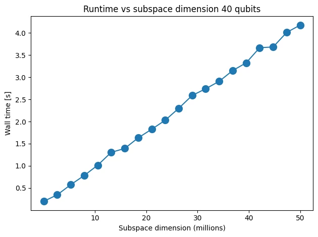
Ora facciamo lo stesso per 60 qubit:

n_qubits = 60
bts_matrix = random_bitstrings(50_000_000, n_qubits)

# We need to sort the bitstrings and just keep the unique ones
bts_matrix = sort_and_remove_duplicates(bts_matrix).astype("bool")

# Final subspace dimension after getting rid of duplicated bitstrings
d = bts_matrix.shape[0]

print("Total number of unique bitstrings: " + str(d))

Total number of unique bitstrings: 50000000

pauli = Pauli("Z" * n_qubits)

# Different subspace sizes to test
d_list = np.linspace(d / 1000, d, 20).astype("int")

# It is better to do this once
row_array = np.arange(d)

# To store the walltime
time_array = np.zeros(20)

for i in range(20):
    int_bts_matrix = bts_matrix[: d_list[i], :]
    int_row_array = row_array[: d_list[i]]
    time_1 = time.time()
    _ = matrix_elements_from_pauli(int_bts_matrix, pauli)
    time_array[i] = time.time() - time_1
    print(f"Iteration {i} took {round(time_array[i], 6)}s")

Iteration 0 took 0.236567s
Iteration 1 took 0.424116s
Iteration 2 took 0.673399s
Iteration 3 took 0.905164s
Iteration 4 took 1.168936s
Iteration 5 took 1.454204s
Iteration 6 took 1.74778s
Iteration 7 took 1.920795s
Iteration 8 took 2.259994s
Iteration 9 took 2.550674s
Iteration 10 took 2.681287s
Iteration 11 took 3.04411s
Iteration 12 took 3.293262s
Iteration 13 took 3.471247s
Iteration 14 took 3.726639s
Iteration 15 took 4.072854s
Iteration 16 took 4.221037s
Iteration 17 took 4.498535s
Iteration 18 took 4.741108s
Iteration 19 took 5.159038s

# Data for energies plot
x1 = d_list
y1 = time_array

fig, axs = plt.subplots(1, 1, figsize=(6, 6))

# Plot energies
axs.plot(x1, y1, marker=".", markersize=20)
axs.set_title("Runtime vs subspace dimension 60 qubits")
axs.set_xlabel("Subspace dimension (millions)")
plt.xticks([1e7, 2e7, 3e7, 4e7, 5e7], [str(i) for i in [10, 20, 30, 40, 50]])
axs.set_ylabel("Wall time [s]")

plt.tight_layout()
plt.show()