Noise and errors
Questa pagina non è stata ancora tradotta. Stai visualizzando la versione originale in inglese.
This lesson will introduce quantum noise and errors, including many of their sources, and drawing analogies with classical errors. Understanding the types of errors that can occur, and the ability to model noise using quantum channels, will be critical to understanding future lessons. Indeed, most methods of error handling require that we know something about the type of noise or errors we seek to reduce or correct.
This video gives an overview of noise and errors and calls out a few computational results. The text below adds more detail and explores some types of errors using Qiskit.
Causes
Classical noise and errors
To understand quantum errors and noise, let’s start with the classical analog. Errors occur in classical computers for a variety of reasons, including multiple mechanisms for spurious charge accumulation, single-event upsets, and slow material degradation. Some of these mechanisms (not all) have analogs in quantum computing and will be instrumental in understanding quantum errors and noise. We briefly review a few of those and then move on to the quantum analogs.
Thermal noise:
As components of a computer heat up, the thermal motion of the atoms and charge carriers changes the resistivity of the material (usually increasing it). This means the resistance in the circuit can vary. Although rare, this can result in a spurious logic transition in a transistor. Although minor variations are inescapable, proper cooling of components is key in avoiding these effects.
Thermal damage and degradation:
Repeated heating and cooling of materials can cause very slow migration of conductive elements (metals). At best, this changes the resistance or capacitance (or both) of circuit elements and leads to imprecise timing in circuit operation. At worst, it results in a short-circuit or hard fault. Again, proper temperature control is key in preventing this type of degradation.
Radiation-induced effects (single-event upsets, SEUs):
Sometimes, high-energy particles can ionize atoms inside a processor and lead to a spurious charge. If it happens at the wrong place and wrong time, this can lead to logical errors. The source of these high-energy particles (including electromagnetic radiation and neutrons) is typically high-energy interactions in the upper atmosphere. These upsets are thus more common in high-altitude environments, including space. These are addressed using error-correcting codes and radiation-hard design.
Electromagnetic interference:
Errors can also be caused by external electromagnetic (EM) fields from switching power lines, radio transmitters, or other system components. This is different from the high-energy radiation in the previous phenomenon. Here, stray time-dependent EM fields induce current and voltage across computing components (as opposed to ionizing a particular atom in one event). Because the time-dependence of fields is a determining factor in the induced voltages, this type of interference is especially important in high-frequency systems. These errors can be combatted through shielding and grounding, among other things.
Crosstalk between interconnects:
Capacitive or inductive coupling between adjacent conductors, especially in nanoscale integrated circuits, can lead to spurious signals. This is related to electromagnetic interference, but it is different because the source of the offending field is another component inside the computer circuit. Think of two wires very close to each other. If wire A experiences a sudden transition (change in voltage) it can induce currents in the adjacent wire B. The exact direction and magnitude depend on circuit layout; it could be a coherent net flow of charge or something closer to eddy currents of charge. But in some cases this can lead to unwanted logical transitions. These crosstalk effects can be mitigated through optimal layout spacing, shielding, and controlled signal rise times.
This is not a complete list, but it is sufficient for us to begin to see parallels with quantum computing. Note that in all the types of unwanted interactions above, the manifestation of the noise as a logical error can only take the form of a 0 becoming a 1, or a 1 becoming a 0. This is all that is permitted in the state space of classical bits.
Quantum noise and errors
In quantum computing, noise and errors are often discussed hand-in-hand, but it is important to recognize the difference. Quantum noise refers to the underlying physical disturbance affecting qubits and quantum systems. It includes all forms of unwanted interactions or fluctuations from the environment, imperfect controls, or hardware defects that cause the quantum state to drift away from the ideal. Quantum errors are the specific deviations or faults in the quantum information that result from the quantum noise. Quantum errors are the measurable or operational manifestations of the noise, and errors include bit-flips, phase-flips, amplitude damping, and more. Both noise and errors can occur in a continuous way. For example, the field used in a quantum gate could be off by 0.1%, 0.15%, or any other fraction. This could result in a phase on a qubit that is incorrect, also by any continuous amount. But you will see that, in practice and especially in error correction, it is common to see errors treated as though they are discrete: grouping the accumulated effects into a discrete bit flip or a single phase rotation. This is useful for correcting errors and characterizing them, but it does not mean that the effect of noise on a qubit is solely a discrete set of errors.
There are many types of noise that affect quantum computers. Some can result in multiple types of errors, while others are paired with specific error manifestations. A complete list is beyond the purposes of this lesson; here is a partial list relevant to the rest of this course, some with parallels to classical computing noise.
Thermal:
The two computational basis states and of a qubit are separated by a very small amount of energy. The exact value depends, of course, on the quantum hardware. For solid-state (fixed-frequency transmon) qubits such as those used by IBM Quantum®, the energy gap between these states is on the order of J, or a few microelectron volts. This energy scale can be related to the frequency via or to a characteristic temperature. Since temperature is related to the average kinetic energy of particles in a sample, we can use the Boltzmann constant to obtain an estimate of the temperature at which average particles would have enough energy to cause a transition:
In order to reduce the chance that thermal interactions cause transitions from one qubit computational basis state to another, the temperature of the qubits must be maintained substantially below 100 mK, ideally closer to 15-25 mK. Any significant increase in temperature above these thresholds would result in totally random state occupation and total loss of quantum information.
This is analogous to the thermal errors that can occur in classical computers, in that they are both thermal in origin — but the temperature scale is obviously different, and so is the mechanism for information loss.
Crosstalk and interference:
Crosstalk in quantum computing refers to any unwanted coupling or interference between qubits or control lines such that an operation or signal intended for one qubit inadvertently affects others. It manifests as errors or correlations between qubits that should ideally be independent.
In superconducting qubit architectures like those used by IBM®, crosstalk can arise from microwave control signals leaking into neighboring qubits, unintended coupling between readout resonators, or flux crosstalk between qubit loops.
Many of the approaches to minimizing crosstalk are incorporated into the design of a quantum computer, such as spacing of qubits and ensuring adjacent qubits have different operational frequencies. There are also software approaches to mitigating crosstalk errors, which will be discussed in later lessons.
Imperfect gate operations:
Operations on qubits are carried out using hardware that has finite precision and which can be subject to noise or other sources of inaccuracy. In particular, microwave pulses of specific durations and with specific orientations are used to implement rotation gates. Say for example that a microwave pulse is to rotate 0.30 radians around the axis. There is finite precision in the orientation, leading to some imprecision in the axis of rotation. Further, there is always a fundamental tradeoff between a pulse frequency and its duration. A very long pulse can have essentially a sinusoidal behavior with practically a single frequency. To form a short packet, one needs a superposition of many frequencies. This is the same tradeoff at the root of the energy-time uncertainty relation, although gate precision is not yet pushing up against these fundamental limits; there is room for improvement.
Quantum-inherent noise:
This last type of noise is quite different from the others; it is not due to errors, but due to the nature of quantum mechanics. Suppose a qubit in quantum state is measured and collapses to an eigenstate ( or ). In a fixed-frequency transmon system, the qubit is dispersively coupled to a microwave resonator whose resonance frequency depends slightly on the qubit state. A microwave probe pulse is sent through the resonator, and the outgoing signal acquires a state-dependent phase shift and amplitude change. This signal is then amplified and measured using classical electronics.
At the quantum level, the measurement signal is carried by a coherent microwave field with a finite average number of photons. Due to the quantum nature of electromagnetic fields, the field quadratures exhibit intrinsic fluctuations. These fluctuations are independent of technical imperfections and arise even for an ideal coherent state. Increasing the average photon number increases the measurement signal, but the fundamental noise level remains finite, so that the distinguishability between outcomes improves only as .
Thus, even if the qubit is perfectly prepared and the measurement chain is ideal, the readout signal corresponding to a given qubit state is not a single fixed value but a distribution that limits how well the outcomes can be distinguished. This overlap represents a fundamental source of uncertainty in the measurement process itself. In practice, while technical noise from amplifiers and other components often dominates, this intrinsic quantum noise sets a lower bound on readout fidelity.
Uncertainty is not error:
These sources of noise are all different from the fundamental uncertainty associated with measurements of quantum states. For contrast, suppose that we have a qubit in a quantum state:
This state has a 64% chance of being measured in the state and a 36% chance of being measured in the state. But a single measurement will only yield a or a — so a single measurement will rarely tell us much about the state prior to measurement. Many measurements are required to obtain detailed information about the state. Out of ten measurements, we might expect six or seven to yield . But it would not be shocking if the first ten measurements all happened to yield (like flipping a fair coin and obtaining "heads" ten times in a row: uncommon, but entirely plausible). If we repeated the measurement 1000 times and always obtained , that would indeed be shocking.
There is therefore uncertainty in our knowledge of the quantum state based on any finite number of measurements. As we repeat the measurements, our knowledge of the quantum state prior to measurement improves, but it is never perfect. One might colloquially say that there is always some underlying "error" in any quantum measurement result. But this is a different use of the term "error" and this is better described as statistical uncertainty. The process of increasing knowledge of a quantum state through many measurements is called quantum state tomography. Quantum state tomography is not limited to measurements along Z, however; it generally refers to measurements along orthogonal axes (like X, Y, and Z) for determination of amplitudes and relative phase. For more on this process, see this section in John Watrous’s course on the General Formulation of Quantum Information, or for a practical implementation, see this teleportation lesson of the course on Utility-Scale Quantum Computing.
Observing errors and their accumulation
In this section, we will use real quantum computers to observe quantum errors and their accumulation under different conditions. In practice, many sources of quantum errors are typically present simultaneously. In order to observe different types of errors in a somewhat isolated way, we will need to use circuits designed for that isolation. Circuits used in applications of quantum computing will look much more complicated.
Let's start with energy relaxation errors.
Energy relaxation () errors
Recall from our discussion of thermal noise that at any non-zero temperature, there is some probability of a quantum system undergoing a transition between energy eigenstates. The relaxation () dominates because it's driven by spontaneous emission (independent of temperature), while low temperature suppresses the competing excitation process. The longer a qubit sits idle, the more time it has to undergo such a transition. The probability that a qubit prepared in the state remains in after a time is given by
Here, the time is an experimentally-determined characteristic time that is different for every qubit, and may even change slightly over time. IBM® quantum computers are benchmarked regularly, so the times that you find listed for qubits on IBM quantum computers should be accurate and up-to-date. A large value of means the qubit remains in the state you prepared longer (on average). Typical values differ across architectures; the qubits in IBM quantum computers often have times on the order of 200-300 , and you can check the latest values on the Compute resources page.
The characteristic time measures something different: the loss of phase information. We will return to this later.
To observe energy relaxation errors, we will prepare qubits in the state, and then intentionally leave them idle for long periods of time. This is the artificial part. In real quantum workflows, you might have a few qubits that sit idle for long periods while processes are carried out on other qubits; therefore, a few instances of such idle times is not artificial.
Let's begin by importing some packages and selecting the least-busy backend.
# Added by doQumentation — required packages for this notebook
!pip install -q cycler matplotlib numpy qiskit qiskit-aer qiskit-ibm-runtime
from qiskit_ibm_runtime import QiskitRuntimeService
import numpy as np
import matplotlib.pyplot as plt

# If your credentials are already saved locally
service = QiskitRuntimeService()

# To load an unsaved instance, uncomment the line below
# service = QiskitRuntimeService(channel = "ibm_quantum_platform", instance = "your crn here")

# To select the least-busy backend:
# backend = service.least_busy(simulator=False, operational=True)

# To specify the backend by name:
backend = service.backend("ibm_boston")

props = backend.properties()
print(backend)
<IBMBackend('ibm_boston')>
Now we will select a qubit to work on, in this case, qubit zero. We can directly import the properties of this qubit, including and .
qubit_idx = 0
qubit_props = props.qubit_property(qubit_idx)

t1 = qubit_props["T1"][0]  # * 1e6  # Convert seconds to µs
t2 = qubit_props["T2"][0]  # * 1e6  # Convert seconds to µs

# print(f"Qubit {qubit_idx}: T1={t1} µs, T2={t2} µs")
print(f"Qubit {qubit_idx}: T1={t1} s, T2={t2} s")
Qubit 0: T1=0.0002737016180018049 s, T2=0.00042784777605680494 s
Knowing in units of microseconds is important, but you might not have an intuitive feel for what that means. After all, gate operations on quantum computers are very fast. The real question is: how much can we do on a quantum computer in that amount of time. To this end, it is useful to relate to other time scales used in quantum computing — specifically to the following:
- sampling time - the smallest clock tick over which control processes can be implemented on the quantum computer.
- single-qubit gate times - the time required to implement a gate operation on a single qubit. This will not be a single value, but a range of possible numbers depending on gate type.
- two-qubit gate times - the time required to implement a gate operation on two adjacent qubits. This can also take on a range of values, but is typically about one order of magnitude longer than for a single-qubit gate.
Let's check for our backend, and display some plausible ranges for gate times.
print(f"Using backend: {backend.name}")

# Access the backend target
target = backend.target

def get_gate_times(target, gate_name):
    results = []

    if gate_name not in target:
        return results  # gate not supported

    # target[gate_name] is a dict: {(qubits): InstructionProperties}
    for qubits, props in target[gate_name].items():
        if props.duration is not None:
            results.append({"qubits": qubits, "duration_ns": props.duration * 1e9})

    return results

# Query some gates
for gate in ["cz", "x"]:
    times = get_gate_times(target, gate)

    print(f"\nGate: {gate}")
    if times:
        for entry in times[:5]:
            print(f"  Qubits {entry['qubits']}: {entry['duration_ns']:.2f} ns")
    else:
        print("  Not available on this backend")
Using backend: ibm_boston

Gate: cz
  Qubits (0, 1): 68.00 ns
  Qubits (1, 0): 68.00 ns
  Qubits (1, 2): 68.00 ns
  Qubits (2, 1): 68.00 ns
  Qubits (2, 3): 88.00 ns

Gate: x
  Qubits (0,): 32.00 ns
  Qubits (1,): 32.00 ns
  Qubits (2,): 32.00 ns
  Qubits (3,): 32.00 ns
  Qubits (4,): 32.00 ns
These gate times will vary from backend to backend. We will hard-code a two-qubit gate time pulled from ibm_boston of 68 ns.
dt = backend.configuration().dt
two_q_gate_time = 68e-9
print("The sampling time is : ", dt)
print("dts per T_1 : ", t1 / dt)
print("2-qubit characteristic time : ", two_q_gate_time)
print("The sampling time intervals per two-qubit gate : ", two_q_gate_time / dt)
print("2-qubit gates per T_1 : ", t1 / two_q_gate_time)
The sampling time is :  4e-09
dts per T_1 :  68425.40450045122
2-qubit characteristic time :  6.8e-08
The sampling time intervals per two-qubit gate :  17.0
2-qubit gates per T_1 :  4025.0237941441897
Keep in mind that no other error sources nor their suppression or mitigation have been taken into account here. errors are not the only errors at work in a quantum system, so don't be too concerned about these numbers. This simply means, in the absence of any suppression, we might plausibly implement on the order of thousands of two-qubit gates before errors start to dominate. Other errors will typically dominate at much lower depths, and conversely errors might still be worth suppressing at much shorter times than those required to wash out the signal entirely.
We will start by using a simulator with a noise model, and then we will compare the results to real hardware.
from qiskit_aer import AerSimulator
from qiskit_aer.noise import NoiseModel, thermal_relaxation_error
from qiskit import QuantumCircuit
from qiskit.quantum_info import Pauli
from qiskit.transpiler import generate_preset_pass_manager
from qiskit_aer.primitives import EstimatorV2

pass_manager = generate_preset_pass_manager(backend=backend, optimization_level=0)
Let us define a time step for our measurements corresponding to the high-end estimate for a two-qubit gate time. Then we will build 50 circuits in increments of that time step. In this way, we will see what happens over a time scale similar to implementing 80 two-qubit gates. Precision here is not critical, so we will use only a handful of shots.
n_points = 50  # We will show 50 steps
delay_unit = 80  # The delay in units of two-qubit-time from above
shots = 100
We build a noise model for our simulator that explicitly includes thermal relaxation errors.
# Create noise model with thermal relaxation for delays
noise_model = NoiseModel()
error = thermal_relaxation_error(
    t1, t2, two_q_gate_time * delay_unit
)  # error model characterized by times in ns
noise_model.add_all_qubit_quantum_error(error, ["delay"])

sim = AerSimulator(noise_model=noise_model)
Now we build our circuits and observables. These are exceptionally simple. The circuits will consist simply of preparing the qubit in and implementing delays for increasing periods of time, using the characteristic gate times and defined above. The observables will simply be , because what we want to know is whether the qubit has remained in or decayed to . Although transpilation is not always necessary for simulators, we go ahead and transpile our circuits here for use later on a real backend.
observables = [Pauli("Z")] * n_points
circuits = []
obs = []
delay_times_sim = []
for i in range(n_points):
    qc = QuantumCircuit(1, 1)
    qc.x(0)
    if i > 0:
        for j in range(i):
            qc.delay(delay_unit * two_q_gate_time, 0, "s")
            j = j + 1
    qc_opt = pass_manager.run(qc)
    circuits.append(qc_opt)
    delay_times_sim.append(delay_unit * two_q_gate_time * i)
    observables_isa = observables[i].apply_layout(layout=qc_opt.layout)
    obs.append(observables_isa)
We run our job using a simulator.
pubs = list(zip(circuits, obs))

# Create AerSimulator with noise model as backend
simulator = AerSimulator(noise_model=noise_model)

# Create SamplerV2 from the AerSimulator backend
estimator = EstimatorV2.from_backend(simulator)

# Run the sampler on the circuit, specify shots
job = estimator.run(pubs)
result = job.result()
Finally we plot the outputs.
# Optional: color palette similar to 'mpl', style = 'clifford'

from cycler import cycler

plt.rcParams["axes.prop_cycle"] = cycler(
    color=[
        "#4C78A8",  # muted blue
        "#72B7B2",  # teal
        "#54A24B",  # green
        "#9C89CC",  # purple
        "#B279A2",  # mauve
    ]
)

# Everything else stays at Matplotlib defaults

# Example data: assume result is a list of objects with structure result[i].data.evs.item()
# and delay_times is already defined as a list of floats.

# Extract y-values
y_sim_values = [(1 - r.data.evs.item()) / 2 for r in result]

# Use delay_times as x-values
x_sim_values = delay_times_sim

# Create the plot
plt.figure(figsize=(8, 5))
plt.plot(x_sim_values, y_sim_values, marker="o", linestyle="-", label="EV Data")

plt.xlabel("Idle Time (s)")
plt.ylabel("Probability of measuring |1>")
plt.title("T1 Decay")
plt.grid(True)
plt.show()
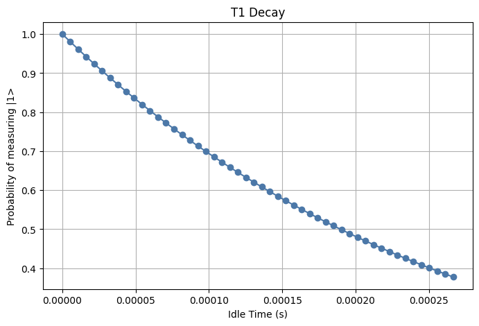
The exponential decay is clearly visible, and in this time, it decays to just under a 40% chance of being in . Note that this is exactly consistent with the model: where we have chosen the maximum to be on the same order as ; recall that we said might correspond to 60 gates (or that order of magnitude), and here corresponds to 60 gates. Thus
Now let's run the same circuits on a real quantum computer. In order to span the same delay duration with fewer jobs, we will increase the delay unit and decrease the number of points.
# This took 27 s on ibm_boston

from qiskit_ibm_runtime import EstimatorV2

# Explicitly use a pass manager with optimization level 0 so that we don't remove the delays
pass_manager = generate_preset_pass_manager(backend=backend, optimization_level=0)

# Use the same time parameters and shots
n_points = 10
delay_unit = 400
shots = 100

# Measure Pauli Z's as your observables
observables = [Pauli("Z")] * n_points
circuits = []
obs = []
delay_times = []
for i in range(n_points):
    qc = QuantumCircuit(1, 1)
    qc.x(0)
    if i > 0:
        qc.delay(delay_unit * two_q_gate_time * i, 0, "s")
    qc_opt = pass_manager.run(qc)
    circuits.append(qc_opt)
    delay_times.append(delay_unit * two_q_gate_time * i)
    observables_isa = observables[i].apply_layout(layout=qc_opt.layout)
    obs.append(observables_isa)

pubs = list(zip(circuits, obs))
estimator = EstimatorV2(mode=backend)
job = estimator.run(pubs=pubs)
result = job.result()

# To print the job id for later retrieval of data
# job_id = job.job_id()
# print(f"Job ID: {job_id}")
Now we plot the results.
fig, ax = plt.subplots()

# Convert from the expectation value of Z to the probability of a transition
y_real_values = [(1 - r.data.evs.item()) / 2 for r in result]

# Use delay_times as x-values
x_real_values = delay_times

# Exponential decay to match theoretical model
t_smooth = np.linspace(0, x_sim_values[19], 100)  # Smooth x-range covering your data
y_decay = np.exp(-t_smooth / (t1))  # y = exp(-t/t1)
ax.plot(t_smooth, y_decay, "k--", linewidth=1, label=f"Perfect Decay (t1={t1:3f} s)")

# Add simulator values
ax.scatter(x_sim_values, y_sim_values, label="Simulator", alpha=0.7)

# Add real QC values
ax.scatter(x_real_values, y_real_values, label="Real", alpha=0.7)

# Add labels and plot
ax.set_xlabel("Idle Time (s)")
ax.set_ylabel("Probability of measuring |1>")
ax.legend()
ax.set_title("T1 Decay")
ax.grid(True)

plt.show()
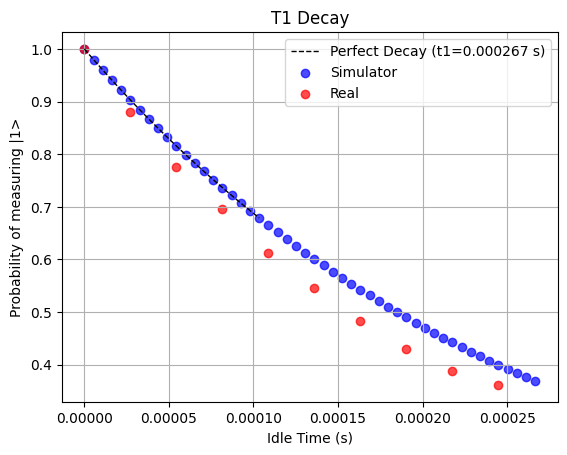
As we can see, the decay of the state over time matches theory (and the definition of ). Further, the simulator is fairly good at matching the behavior of the real quantum computer in this case. Here are a few things to keep in mind about the decay of this state:
- We have artificially delayed measurement for an unrealistic amount of time. These delays correspond to the timescale of extremely deep circuits that could consist of thousands of two-qubit gates. This was done only to show that the effects of thermal noise exist. In real circuits applied to real-world problems, operations would be performed on other qubits while a handful might sit idle long enough for energy relaxation errors to matter — but other errors would dominate before reaching a full .
- No error mitigation or suppression techniques have been used. We can alter this decay curve by using techniques we will learn in this course.
- We used only 100 shots here, which is unusually low because we sought only to demonstrate that the effect exists. You will likely use more than 1,000 shots in applications.
This first visualization of error required almost no gates other than delays (and the single X gate used to prepare ). Let us now look at another example that focuses on gate error.
Gate errors and accumulation
When we apply a quantum gate, say an gate, theoretically that gate rotates a quantum state by angle radians about the axis on the Bloch sphere, mapping to via
However, a real gate is imperfect. It might be imperfectly oriented (causing rotations not perfectly about the X axis) or it might cause a slightly greater or smaller rotation than intended. Let us model a gate error as being purely over/under rotation by a small angle .
If an imperfect gate is applied many times, small errors can compound. Sometimes these multiple errors even cause the state to shift in the same direction each time (a phenomenon called "coherent accumulation", which we will revisit below). Let's see what happens when we apply a real X gate to a qubit many times.
# This took 78 s on penguino1

from qiskit_ibm_runtime import EstimatorV2

# Explicitly use a pass manager with optimization level 0 so that we don't remove the delays
pass_manager = generate_preset_pass_manager(backend=backend, optimization_level=0)

# Use the same bit flips
max_depth = 60
circuits = []
observables = []

for depth in range(max_depth + 1):
    qc = QuantumCircuit(1)
    # Repeat flipping back and forth depth times
    for _ in range(depth):
        #    qc.x(0)
        qc.x(0)
        qc.barrier()
        qc.x(0)
        qc.barrier()
    circuits.append(qc)
    observables.append(Pauli("Z"))

pubs = list(zip(circuits, observables))

estimator = EstimatorV2(mode=backend)
results = estimator.run(pubs=pubs).result()
real_expectations = [pub_res.data.evs for pub_res in results]
# from qiskit_ibm_runtime import QiskitRuntimeService

# service = QiskitRuntimeService()           # uses stored IBM Quantum account
# job_id = "d5immof67pic7386l8eg"

# job = service.job(job_id)                 # retrieve the job
# results = job.result()                        # this is your .result() object
# Convert from the expectation value of Z to the probability of a transition
# y_real_values = [(1-r.data.evs.item())/2 for r in results]

# Create the plot
plt.figure(figsize=(8, 5))
# plt.plot(range(max_depth + 1), y_real_values, 'o-')
# plt.plot(x_real_values, y_real_values, marker='o', linestyle='-', color='blue', label='EV Data')
plt.plot(
    range(max_depth + 1),
    real_expectations,
    marker="o",
    linestyle="-",
    color="blue",
    label="EV Data",
)

plt.xlabel("Number of Flip-Back Cycles")
plt.ylabel("Expectation ⟨Z⟩")
plt.title("Accumulated Gate Noise Effects on Flips")
plt.grid(True)
plt.show()
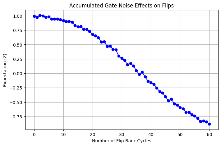
The expectation value starts out around 1.0 as expected, and decays, but it doesn't just decay to zero! It becomes negative. If this were thermal noise or random interactions, it would not make more likely to be measured than . This error is clearly different. And it makes sense in the context of our over/under-rotation discussion. If each rotation pair that should cancel actually ends up rotating by a small angle, then many such repetitions would slowly allow the state to rotate from toward .
The accumulation of errors shown here is not likely to proceed as cleanly in a real workflow. For one thing, we have explicitly turned off error mitigation and performed the same repetitive gate sequence to allow errors to accumulate coherently. This is done solely to demonstrate that these errors exist. When we use noise-handling techniques (for example, Pauli twirling), we can influence how error accumulates, often yielding lower overall error.
We can check exactly how well our model of this error fits the experimental data by building a noise model explicitly and using a simulator. In the model below, we explicitly build in an error corresponding to 0.025 radians. That is not a magic number; one can simply tune the error until it reasonably describes the experiment.
from qiskit_aer.noise import NoiseModel, coherent_unitary_error
from qiskit_aer import AerSimulator
import numpy as np

# For your SINGLE-QUBIT test on qubit 0, just override X error specifically
noise_model = NoiseModel.from_backend(backend, gate_error=True, thermal_relaxation=True)

theta_error = 0.025  # model over-rotation error around 0.01-0.03 radians
U_over = np.array(
    [
        [np.cos(theta_error / 2), -1j * np.sin(theta_error / 2)],
        [-1j * np.sin(theta_error / 2), np.cos(theta_error / 2)],
    ]
)

unitary_error = coherent_unitary_error(U_over)
# Target ONLY qubit 0 (your circuit) - no warning!
noise_model.add_quantum_error(unitary_error, ["x"], [0])

simulator = AerSimulator(noise_model=noise_model)
WARNING: quantum error already exists for instruction "x" on qubits (0,) , appending additional error.
max_depth = 60
circuits = []
observables = []

for depth in range(max_depth + 1):
    qc = QuantumCircuit(1)
    # Repeat flipping back and forth depth times
    for _ in range(depth):
        #    qc.x(0)
        qc.x(0)
        qc.barrier()
        qc.x(0)
        qc.barrier()
    circuits.append(qc)
    observables.append(Pauli("Z"))

pubs = list(zip(circuits, observables))

estimator = EstimatorV2.from_backend(simulator)
results = estimator.run(pubs).result()
expectations = [pub_res.data.evs for pub_res in results]  # no [0], use value directly
Now we can plot the real and simulated curves together.
fig, ax = plt.subplots()

# Add simulator values
ax.scatter(range(max_depth + 1), expectations, c="blue", label="Simulator", alpha=0.7)

# Add real QC values
ax.scatter(range(max_depth + 1), real_expectations, c="red", label="Real", alpha=0.7)

# Add labels and plot
ax.set_xlabel("Number of Flip-Back Cycles")
ax.set_ylabel("Expectation ⟨Z⟩")
ax.set_title("Accumulated Gate Noise Effects on Flips")
ax.legend()
ax.grid(True)

plt.show()
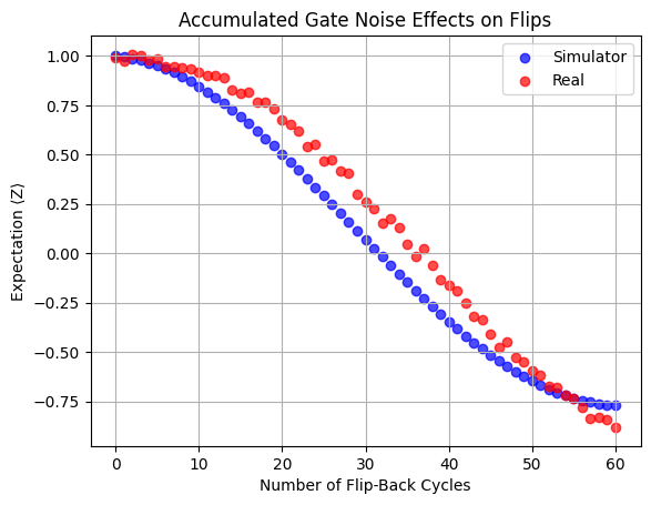
The error in the real circuit was fairly well described by the over/under-rotation error model. Clearly different kinds of noise and errors will accumulate differently and result in drastically different effects on the fidelity of our quantum circuits. It thus becomes very important to classify and characterize the errors that can occur more formally than we have thus far.
Characterizing quantum errors
We have already described some of the sources of quantum noise, and we could categorize errors according to the categories of noise that cause them. But there could be different categories of quantum errors that are useful in error correction and mitigation. For example, we need to know at what point errors occur and how errors accumulate if we want to correct or mitigate them. In specifying where (in what processes) errors occur, a common important category is state preparation and measurement errors (or SPAM errors, for short). Here, the term “state preparation” does not mean everything that is done on a state preparing it for measurement. Rather, it refers to initialization of the qubits, the “preparation” of the qubits for the execution of an algorithm, and so this SPAM category excludes things like gate errors during algorithm execution.
Another important distinction is whether the errors are coherent or incoherent. To summarize briefly (we discuss them more in detail below), coherent errors are typically modeled by unitary operations and preserve state purity. Incoherent errors are modeled by non-unitary quantum channels and generally reduce state purity. It’s easy to visualize incoherent errors as thermal interactions that cause loss of quantum information, but really they could be caused by any random coupling to the environment. For an example of a coherent error, suppose there is an imperfection in pulse orientation in implementing an RY gate such that an gate actually causes . Such an imperfection would always cause an erroneous rotation around X in the same direction. This would be a coherent error.
Note that SPAM errors include a mix of coherent errors, like systematic control faults, and incoherent errors, such as photon loss and thermal effects. Because this involves multiple steps and error sources, SPAM errors are best described as a combination of both coherent and incoherent errors.
SPAM errors
As the name suggests, SPAM errors arise at two distinct stages of a quantum experiment: initial preparation and readout/measurement. State preparation errors occur when the hardware fails to reliably initialize qubits in the desired starting state ( for IBM quantum computers). Causes include:
- thermal excitation (real qubits are not perfectly cooled and can occasionally start in instead of )
- residual photons or noise in resonators in superconducting qubits
- drifts in calibration that affect how accurately qubits are reset
Measurement errors occur during the readout process, when the measurement apparatus misidentifies the qubit state. Sources include:
- readout amplifier noise causing confusion between and
- qubit relaxation during readout (for example, a qubit in decays to just before or during measurement)
- crosstalk between readout lines: reading one qubit slightly influences readings on neighboring qubits
- Imperfect discrimination thresholds in the IBM resonator-based measurement systems
SPAM errors are primarily incoherent. Preparation errors act like random mixtures of excited and ground states. Measurement errors behave like classical confusion: with probability , is reported as or vice versa. These are distinct from coherent unitary errors (like miscalibrated gates causing systematic phase shifts). SPAM errors instead resemble random classical noise, though rare coherent biases in readout can exist.
SPAM errors can be problematic for randomized benchmarking or for short-depth circuits where state preparation and measurement represent a large fraction of total error. They are less of an issue for very deep circuits, especially those with many two-qubit gates.
Mathematically, SPAM errors can be described as producing a noisy distribution that is related to the ideal distribution through a matrix :
Here is the probability of measuring bitstring , and is the probability of obtaining state when the state should have been prepared in state . Picture the context of sampled bitstrings from Sampler. Your measured distribution of states will consist of many accurate measurements, but also some measurements in which instructions for state preparation do not match the observed state. This means the probabilities will be slightly off.
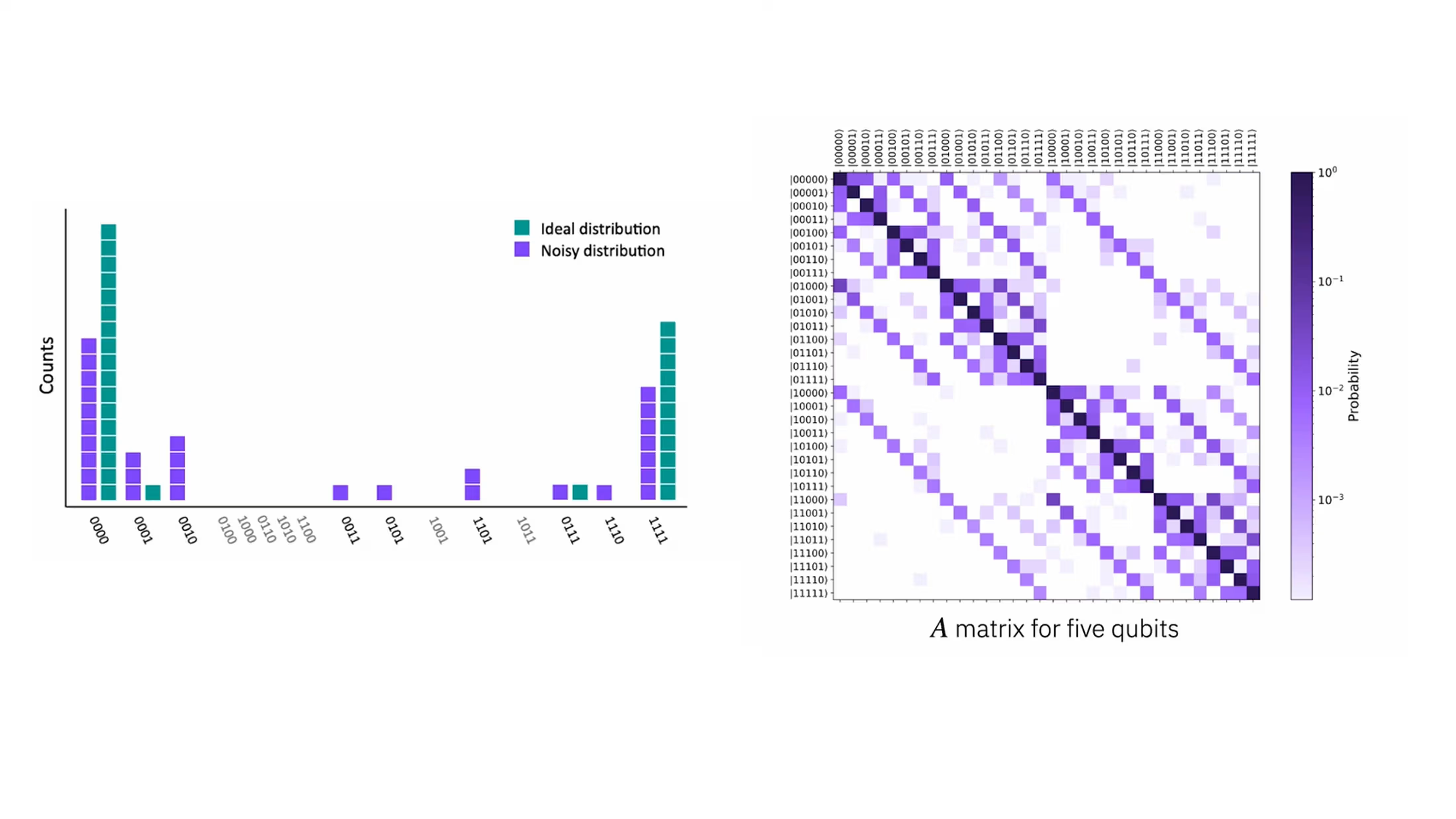
In the figure above, part (a) shows the ideal distribution of a GHZ state in teal, and the actual measurements in purple. In part (b) we see an example of an matrix. Note that the matrix is not perfectly symmetric across the diagonal, since each qubit need not be equally likely to erroneously return a 0 and to erroneously return a 1. In practice, it is often hard to separate preparation and readout errors, so they are often combined in a single treatment (hence the common use of SPAM).
One way of correcting these SPAM errors is by using simple circuits with known ideal measurement outcomes and comparing those to the measured outcomes in the presence of SPAM errors. This can be used to reverse-engineer the ideal outcomes of more complex circuits. For general high-entropy states, this could require constructing a matrix with probabilities, but in less extreme cases these errors can be mitigated.
Coherent errors versus incoherent errors
Coherent errors are systematic, deterministic, and unitary mis-rotations of the quantum state. They arise from imperfect quantum operations that deviate in a predictable way. Examples include slight errors in rotation applied by single-qubit rotation gates, including those caused by calibration drift which would consistently over- or under-rotate. Mathematically, we could write that a real rotation gate, say is given by the ideal rotation gate plus some additional error:
for some small under- or over-rotation . Other examples include a two-qubit gate adding a small unwanted phase shift and control pulses that systematically deviate from the ideal shape.
A key characteristic of coherent errors is that they are deterministic and can be modeled by unitary gates, themselves. Correspondingly they preserve the purity of the quantum state: the quantum information is not lost, it has simply been processed imperfectly. Another important point to note is that repeated coherent errors interfere constructively and sometimes grow quadratically with the number of gates.
These errors are sometimes predictable and can thus be calibrated away to some extent. But the coherent errors that remain may accumulate quickly, causing troublesome deviations from ideal states. This means that sometimes it is advantageous to intentionally "randomize" coherent errors. This procedure and its usefulness will be covered in the lesson on error mitigation.
Why they are troublesome
Coherent errors can “pile up” in dangerous ways, producing large deviations from the correct state if not randomized or corrected.
Incoherent errors are stochastic, random, and often non-unitary. They arise from interactions with the environment or uncontrolled noise sources. We have already seen some examples: energy relaxation / decay is incoherent. So are stochastic gate noise, thermal noise, and measurement error.
The key feature of incoherent errors is that they are not the same each time an operation is performed. They are non-unitary, so they cannot be modeled by a simple unitary quantum gate as coherent errors could. Because they are incoherent, they typically accumulate in a linear way like random noise, not like a consistent over-rotation.
Incoherent errors cause qubits to lose information irreversibly (loss of purity and phase information).
So which is worse? As with most things in quantum computing, it depends. The takeaway is that coherent errors accumulate faster and non-linearly (which is bad). But they can be partially calibrated away and the phase information is still there in your system, if you can figure out how to properly extract it. Incoherent errors accumulate linearly, which is good for two reasons: it is slower than coherent accumulation and it is fairly easy to see how effects of incoherent errors scale for processes like zero-noise extrapolation (ZNE), which will be covered in the lesson on error mitigation. However, when incoherent errors occur, quantum information is truly lost, not merely obscured.
Density matrices and quantum channels
In the following sections, we will go deeper into a few types of coherent and incoherent errors and see how they can be modeled mathematically using quantum channels. First, a brief refresher on density matrices and quantum channels is in order. For a full, rigorous treatment of these, see John Watrous's course General formulation of quantum information on IBM Quantum Learning. The treatment here will be example-driven and less formal.
Quantum channels are the most general way to describe how a quantum system evolves, interacts, and undergoes noise. If you’re used to pure states and unitary evolution, quantum channels are the natural next step.
In standard quantum mechanics, a "pure" state is written as . Here "pure" refers to purity of information or knowledge of preparation of the state; it does not mean an eigenstate of some system. For a qubit example, is a pure state because we have perfect knowledge of the relative amplitudes and phase. The time evolution of such a pure state is governed by a unitary operator :
as per the Schr"odinger equation, in which , where is the system Hamiltonian and is the reduced Planck's constant, often "set equal to one" or more rigorously, absorbed into the Hamiltonian so that all energies are given in units of .
Unitary evolution is reversible, deterministic, and isolated. But this is inadequate to describe real quantum systems. In real quantum systems:
- We perform measurements, collapsing the quantum state into an eigenstate of the system. This is explicitly non-unitary.
- The system interacts with an environment. This means the system is not truly isolated, and since the environment cannot be tracked ad infinitum it corresponds to loss of information.
- Practically speaking: noise corrupts the state. And more.
Unitary evolution alone cannot describe these processes; therefore, we need a more general representation of quantum states and processes. A mixed state describes a classical distribution of quantum states. That is, we are already familiar with the fact that the quantum state: has a 50% chance of being measured (collapsed into classical information) in the state and a 50% chance of being measured in . But the claim is that the initial quantum state is exactly with 100% probability. Now we want to add on top of the quantum mechanical probability a classical probability, for example:
The initial quantum state is prepared in with a 25% classical probability, and is prepared in with a 75% classical probability (note the different relative phases).
Sometimes this can be due to explicit classical probabilities in preparation; other times it can be due to entanglement with parts of the environment that we ignore. Either way, the need is clear for a tool to describe this classical distribution of quantum mechanical states. Pure states alone cannot represent these possibilities. Therefore, we introduce the density matrix.
A mixed state is described by a density operator:
Here, is a quantum state (not necessarily an eigenstate of any particular operator) and is the classical probability that the system is prepared in the state . This is a good prescription for how to build a density matrix from a known classical distribution of quantum states. On the other hand, we might want to know given both a classical distribution of quantum states and a quantum mechanical probability of different measurement outcomes, what is the probability that a measurement yields a particular state (like , or , or other states when more qubits are involved). That is where the density matrix is especially useful. We can also write it in a basis as:
Here the diagonal elements are probabilities:
- = probability the qubit is in
- = probability the qubit is in
They are real, non‑negative, and sum to 1.
Off-diagonal elements are coherences: phase relationships or interference capability, and generally correspond to how much quantum mechanical information is in the state. This is an informal statement, but let's see what it means in practice.
Example
Consider the pure state . (a) What do you know about probabilities of measurement and phase information without doing any math? (b) Build the density matrix and verify your intuition.
Solution:
(a) Because it is a pure state, there is only one possible phase between and : +1. This is perfect phase information, so we expect off-diagonal elements in our density matrix to be large. You might have more intuition than that about the off-diagonals, but that is sufficient for now. Further, the amplitudes of the two basis states are equal, so we expect a 50% probability of measuring either or . So we expect the diagonal entries to be 1/2. (b) Using the definition above:
only for the state . So we can write
The diagonal entries are each as expected, and the off-diagonal elements are large (sum to one).
Now let's see what happens when we do not have good phase information.
Example
Consider a similar case, but now with a 50% classical probability of being in the state and a 50% classical probability of being in the state . Same two questions: (a) What do you know about probabilities of measurement and phase information without doing any math? (b) Build the density matrix and verify your intuition.
Solution:
(a) As before, the amplitudes of the two basis states are equal, so we expect a 50% probability of measuring either or . So we expect the diagonal entries to be 1/2. But this time there are two opposite possibilities for the phase between and : +1 and -1, and each one is equally likely. One might expect that with two equally likely opposite phases, one has little to no phase information. One might expect the off-diagonal entries to be small. (b) Again using the definition above
only for the two states and . So we can write
The off-diagonal entries are small, zero in fact, as expected. The diagonal elements are still 50% each, which makes sense because each of the states in the mixture had and equally weighted.
This construct becomes more interesting as the number of qubits increases. Explore this in the questions below.
Check your understanding
Write the density matrix for the pure Bell state .
Answer
only for the state . So we can write
Write the density matrix for a 25% classical probability of and a 75% classical probability of .
Answer
only for the two states and . So we can write
Modify your work from the previous question to write the density matrix for a 50% classical probability of and a 50% classical probability of . Predict what phase information should persist.
Answer
only for the two states and . So we can write
The diagonal terms sum to 1, as they must. The off diagonal terms do not cancel here as they did in a previous, one-qubit example. You can see why, in the math, but a short-hand explanation is that there are more states in our Hilbert space now. Although the first Bell state had a positive relative phase and the second had a negative one, these phases were between different basis states. The first Bell state had a phase between and , while the second had a relative phase between and .
Quantum channels
A quantum channel is the most general physically allowed transformation of a quantum state. It takes an initial density matrix to another density matrix:
Here means a quantum channel acting on a density matrix , not to be confused with the Bell states or .
Quantum channels are extremely general. They can include:
- Unitary evolution
- Probabilistic mixtures of unitaries
- Measurements
- Decoherence
- Amplitude damping (energy loss)
- Dephasing (loss of phase information)
- Interaction with an environment And many other things.
One way of thinking about quantum channels is that they are to density matrices what unitaries are to pure states. But the generality of density matrices allows the corresponding quantum channels to be much more general and thus more powerful.
The only constraints on a quantum channel are that it must be:
- Linear Mixtures of states should evolve consistently:
- Completely positive It shouldn’t produce negative probabilities, even if your system is entangled with something else.
- Trace-preserving Probabilities must add to 1. These are sometimes collected together in the acronym CPTP: Completely Positive Trace-Preserving maps.
There are different representations of quantum channels, including Stinespring, Kraus, and Choi representations. These are treated in detail in this lesson on quantum channels in General formulation of quantum information and they are also shown there to be equivalent. We will not get into these different representations here. Suffice it to say that they are analogous to describing vectors using three different coordinate frames. Each might emphasize different aspects and build intuition in a different way; but they all give you the correct answer. Kraus representations are convenient for our purposes. They offer a convenient formulaic way to express the action of a channel through matrix multiplication and addition. In particular, a Kraus representation is a specification of a channel, , in the following form.
Here, are matrices that all have the same dimensions: their columns correspond to the classical states of the input system, , and their rows correspond to the classical states of the output system, whether it's or some other system . In order for to be a valid channel these matrices must satisfy the following condition.
These matrices are called Kraus matrices. This formulation is applicable not only to noise channels, but to general quantum processes and channels, including measurement. Let's see an example of how these can be used to build channels in the context of noise and errors.
Completely dephasing channel
Consider a channel that destroys all phase information and call it the completely dephasing channel. This means the channel should take any density matrix of the form
and map it to
If we assume that the density matrix has already been written in the computational basis, we can express as . This suggests a set of Kraus matrices that can accomplish this channel action: . Let's apply this strategy to an example case of a single qubit, and see if it works as we require:
Set and
Because is a number, we can simply move the vector past it. This applies to the second term as well. We have:
Note that these matrices satisfy the required condition:
It is worth noting that this choice of Kraus matrices is not unique.
Characterizing noise as channels
In this section we will use the model of the Bloch sphere and the mathematics of quantum channels to better understand various types of noise and errors.
Incoherent errors
Let us return to incoherent errors and specifically explore energy relaxation errors. Recall that the state is a qubit's ground state and the state has a slightly higher energy. Sometimes quantum states will simply spontaneously decay from a higher energy level to a lower one. The process of spontaneous emission is a rich topic and cannot truly be understood without a quantum field theory treatment. But the intuition is very familiar to all of us: random perturbations may cause a rock to tumble down a hill; they will not cause a rock to tumble up a hill. How long a qubit remains in the higher energy state is characterized by a time . More specifically, the probability that a qubit prepared in the state remains in that state after time is . Or, equivalently, the probability of an energy relaxation error after time is
To describe this with a quantum channel in the Kraus representation, we need Kraus matrices that correspond to
- leaving states unchanged
- changing states to with some probability p.
Let us define
First, let us check that this has the desired effects on a density matrix. Consider a system that is in a pure state . We saw in an example above that the density matrix for this case is
Applying the energy relaxation channel using Kraus matrices, we obtain the new, mapped density matrix:
Let's examine this and compare it with our intuition:
First, let's check the limit as approaches zero. We recover our initial density matrix, as we should:
As time passes, we would expect the probability of measuring state to increase, and the probability of measuring to decrease. This is again, exactly what we see, since
We can also trivially see that the probabilities of measuring and sum to 1, as they must.
The precise scaling of the coherence (off-diagonal) terms is beyond the scope of this treatment. But what is clear that we initially have perfect phase information, and after a very long time there can be no phase information since the system is entirely relaxed into the state . Therefore, the coherence terms must decay to zero at very long times. Indeed,
Many of the constraints on our Kraus matrices are implicitly checked through these intuitive considerations. One should rigorously check that the constraints on channels (and on Kraus matrices specifically) are satisfied, but we leave that as an exercise to the reader.
Graphically, this type of channel can be represented using a Bloch sphere. A pure state lies on the surface of a Bloch sphere. Mixed states shift to the interior of the sphere and spread away from a single point. The inclusion of classical probabilities is seen through reduction in the absolute distance from the origin to any one of the states in the mixture, and the spreading from a single point to a region indicates the mixing of multiple possible states. In the special case of an energy relaxation channel, the mixed state (density matrix) after some non-negligible time would look like the image below: a region in the interior of the Bloch sphere, shifted upward toward the pole, and shrunken both along the axis, as well as along the plane, though to a lesser extent than along .

Note that the region is not a "cap" to the Bloch sphere, as it sometimes appears in a perspective rendering. As can clearly be seen in the video, it is an oblate spheroid, shrunken and shifted toward the state. Noise channels (and channels in general) are of course applicable to systems of any size. But representing them visually (as with a Bloch sphere) becomes difficult as the number of mutually orthogonal states in the Hilbert space increases.
Check your understanding
Verify that the Kraus matrices used in the energy relaxation channel above satisfy the identity condition:
Answer
We will present two more types of incoherent noise channels, but we will leave most of the interpretation and verification as exercises. The next is the dephasing channel, which describes a loss of phase information, but with the preservation of amplitudes. Although one can still have both classical and quantum mechanical probabilities involved in overall measurement probability, the loss of phase information is often described as a loss of quantum information, or as the system becoming more classical.
In much the same way energy relaxation was described with a characteristic time , dephasing errors are described by a second time parameter . The probability of a dephasing error after time is given by
A set of Kraus matrices for the dephasing channel on a single qubit, in terms of this probability, are as follows:
The result of this dephasing channel is visualized using a Bloch sphere in the figure below.

Note that the amplitudes are not changed, so any states falling exactly on a pole ( or ) are unaffected and are still mapped to the sphere's surface in the shaded region. But phase information is lost, which corresponds to a shrinking of the shaded region across the plane. A way to make sense of this is: any possible quantum state may still have a well-defined phase, but since there is a classical probability of finding several states with different well-defined phases, the overall probability of any one well-defined phase is reduced.
Check your understanding
Verify that the Kraus matrices defined above for the dephasing channel satisfy the identity condition:
Answer
Start with a single-qubit pure state of your choosing, with a well-defined phase between and . Write it as a density matrix. Apply the dephasing channel using the Kraus operators suggested above. Interpret the resulting, mapped density matrix.
Answer
Let us choose the state . The corresponding density matrix is
Now we apply the dephasing channel to this density matrix using the Kraus operators.
Firstly, we note that the sum of the diagonals is indeed equal to one, as it must be. Secondly, note that the off-diagonal elements were initially large, with a sum of 24/25, indicating strong coherence. Note that as the probability of a dephasing error increases, these off-diagonal elements decrease. This also matches our expectation. One subtlety: note what happens as . The coherence again becomes strong! This seems counter-intuitive at first, because a high probability of a dephasing error should mess up our phase, right? The catch is that if we are 100% sure that a phase error occurs, then we again have strong information about the phase; the phase has simply flipped. With this insight, we might expect the worst phase information to correspond to a 50-50 chance of a phase error occurring, and that is indeed what we find.
Our final example of a noise channel describing incoherent errors is the Pauli noise channel. This channel describes the occurrence of three types of errors with independent probabilities:
- Bit-flip error (X error) with probability
- Phase-flip error (Z error) with probability
- Combined X and Z (Y error) with probability Here, for all . A corollary is that the probability of no error occurring is .
The Kraus operators for this channel are:
In the case of the Pauli noise channel, it is instructive to write out the channel itself:
We see from this form that the Pauli noise channel implements one or more errors corresponding to the action of Pauli matrices , each with probability .
Various combinations of flip probabilities will produce different visualizations. Here we visualize the special case where , also called the depolarizing channel.

Modeling coherent errors
Quantum channels can represent both coherent and incoherent errors, but in practice they are used mainly for incoherent errors because coherent errors are better modeled as unitary miscalibrations or converted into stochastic channels for easier analysis. In this section we will introduce approaches more applicable to coherent errors.
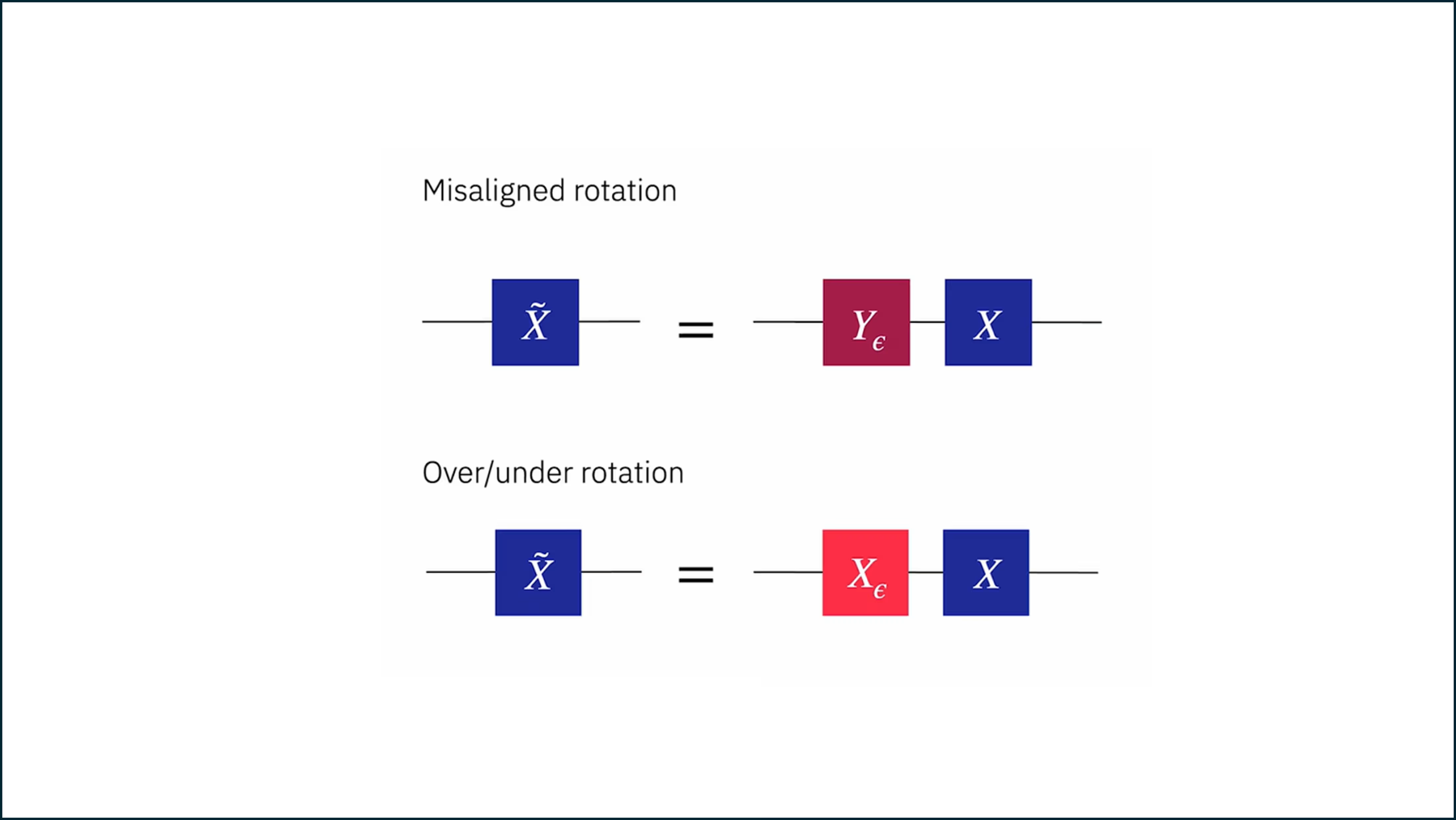
Coherent errors can be modeled by unwanted unitary gates. Some simple examples include misaligned rotations or under-/over-rotation. In the image below, we show a misaligned rotation as an extra rotation by a small amount in addition to the desired rotation about the axis. An over-rotation is described by the desired rotation and also some additional rotation around the same axis .
Two-qubit errors and shaded light cones
A single‑qubit gate rotates an isolated qubit. A two‑qubit gate implements logic relying on two qubits, but cannot make a direct measurement of either qubit; it must therefore turn on an interaction between qubits. This interaction is the reason we can build entanglement, and it’s also where much of the noise, crosstalk, and calibration difficulty comes from. This interaction between qubits also allows errors to spread. If one qubit has some error, and it serves as the control qubit for another target qubit, the error can be passed onto the target. In this lesson we will review what two-qubit gates mean for error rates and their spread within a circuit.
Echoed cross-resonance gates
Different hardware architectures and gate families engineer that interaction in different ways. IBM quantum computers implement abstract two-qubit gates like CZ or CX gates using hardware-native echoed cross-resonance (ECR) gates. ECR gates generate an effective interaction using a microwave drive. Related gates like CNOT are built from by adding single‑qubit rotations.
Different qubits have different resonant frequencies (frequencies to which they react strongly). A standard operation might use that resonant frequency to induce a transition in a qubit. But what happens if you drive qubit C at the resonant frequency of an adjacent qubit T? Adjacent qubits are linked by a fixed capacitive or resonator‑mediated interaction. Due to this coupling, a drive on qubit C “leaks through” into the Hamiltonian of qubit T. The strength and direction of this effective drive depend on the state of qubit C ( or ). Here, qubit C is the control and qubit T is the target.
The result is an effective target‑qubit rotation conditioned on the control qubit’s state. Mathematically:
This ZX interaction is exactly what you need to build a CNOT. But the other terms might include some errors, and are almost certain to include capacitive coupling between qubits C and T, which corresponds to a ZZ term.
We can think about these additional terms in the following way:
- IX = target gets unintentionally driven
- ZI = control qubit acquires an unwanted Z rotation
- IZ = target qubit acquires an unwanted Z rotation
- ZZ = static state‑dependent phase shift
- others = small XY, XX, higher‑order interactions
An ECR gate is simply a controlled rotation plus a carefully chosen echo pulse on the control qubit. The echo flips the sign of many unwanted terms while preserving the ZX interaction. This process cancels IX and ZI errors pretty well, and sometimes some higher-order terms. But echoing cannot cancel the static ZZ coupling because it commutes with the echo pulse. There are other interactions that will not cancel in this process: some residual nonlinearities and spectator‑qubit effects, leakage and long‑range drive contamination, plus a few others — but the ZZ term is especially important.
This process often requires drive times that are an order of magnitude longer than single-qubit gates. The combination of longer drive times, persistent ZZ terms in the Hamiltonian, and imperfections in coupling make two-qubit gates the dominant source of gate errors. Note also that if one needs interactions in a circuit between qubits that are not adjacent, the necessary SWAP gates are also obviously two-qubit gates. This is why the standard depth-related metric is: two-qubit, transpiled depth. We care mostly about two-qubit gates because they dominate gate error, and we need to look at the transpiled circuits because transpilation will often introduce many additional two-qubit gates in the form of SWAP gates.
Check your understanding
Explain why we care mostly about two-qubit transpiled depth. Make sure to consider hardware constraints, and the fact that single-qubit gate depth might be much larger.
Answer
Two-qubit gates have much higher error rates than single-qubit gates. Single-qubit gates are not perfect, so there can be cases in which also considering single-qubit depth is useful. But two-qubit gate depth tends to dominate the error behavior of a circuit. We must consider the transpiled circuit. Modern quantum computers do not have all-to-all qubit connectivity. IBM quantum computers either use a square lattice or a "heavy hex" lattice, meaning qubits have 2, 3, or 4 nearest neighbors to which they can be directly coupled using a single two-qubit gate. Any entanglement with other, non-adjacent qubits requires moving information around on the quantum computer using two-qubit SWAP gates. Thus, transpilation tends to increase two-qubit gate depth. For highly-entangling circuits, this increase could be very large.
Shaded light cones
Assume that a single qubit is well-isolated from all others. An error on that qubit will not cause any errors on any other qubits. But when a qubit interacts with another, errors can propagate. The way errors propagate depends on the way qubits interact. Consider the circuit below. Assume that any qubits adjacent in the circuit diagram are also adjacent in the quantum chip (that is, information will not need to be swapped around to other qubits to facilitate the interactions described).
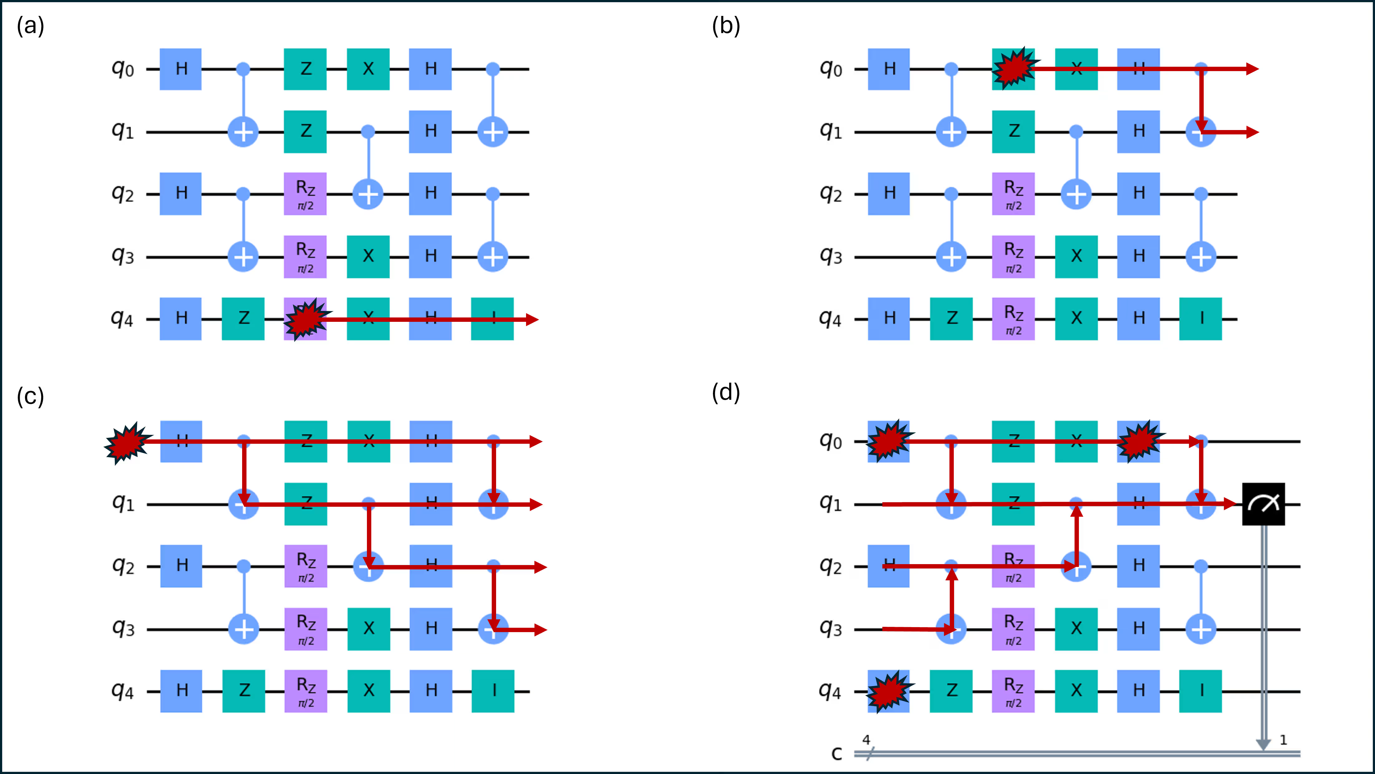
Although you might not have thought of it this way, this is a sort of a spacetime diagram. The vertical axis on a quantum circuit represents different qubits arranged in space. The horizontal axis represents the time over which a sequence of gates are applied. Borrowing language from relativity, a light cone represents the region of spacetime that is reachable from a point via causal interactions.
In the figure above, the type of error has not been specified. It turns out that the type of error affects the light cone since some errors affect the logic of a two-qubit gate, and others do not. We will return to this shortly. For now, consider the yellow lines to be paths of potential spread of some error type. Observe, for example in part (a) of the figure, that a single-qubit error on the RZ gate in qubit 4 can only propagate forward in time on that one qubit. It cannot spread to other qubits because qubit 4 is not entangled with any other qubits. This is a good time to note that qubit 4 is fairly useless in this circuit, and indeed the entire circuit is built for pedagogical purposes only.
An error on the Z gate of qubit 0 (not necessarily a Z-error, just some error at that location), however, could propagate to another qubit: qubit 1, via the final CNOT that uses qubit 0 as the control and qubit 1 as the target. This is shown in part (b). As you might expect, an error earlier in the circuit will often have a chance to propagate across more qubits. Part (c) shows that an error in the initial state preparation of qubit 0 can spread to all qubits except qubit 4, which is isolated.
This setup shows how an error can propagate forward in time to affect measurements. But you can also examine the inverse question: for a specific single-qubit measurement, which parts of my circuit could have contributed some error to it? In that case you would simply start with the measurement or other point of interest and work backwards (in time) through the circuit, following any entangling circuits as shown in part (d). Also shown are a few randomly-chosen points for errors to occur.
In the figure above, errors spread between qubits via ECR gates, but a similar discussion could apply to other two-qubit gates. These gates have a control and a target. It is clear that an error on the control can affect the logic of the gate and can thus result in an error on the target. But what about the other direction? Can an error on the target propagate to the control qubit? Recall that the coupling between control and target for ECR gates is not purely the ideal ZX type; it also has an unwanted ZZ coupling.
If an error on the target commutes with the ZZ coupling, then it cannot propagate to the control qubit. We can see this through the physical mechanisms at work. A quick way to see it is that if an error commutes with , then their order can be swapped without affecting the outcome. However, if occurring just before the coupling is the same as it acting after the coupling, then it cannot affect the control, since in the latter case, the error would have to move backward in time. If an error does not commute with the ZZ coupling, then it might indeed propagate from the target back to the control. Thus, in the case of an ECR gate, Z errors could not propagate from target to control, but X or Y errors could.
Check your understanding
In part (d) of the figure above, look at the vertical lines between qubits 0 and 1. Is it correct that some errors could spread across those lines? Again, it can depend on error type, and we have not discussed this yet. The question is whether any error exists that could propagate as shown by those vertical lines. Explain.
Answer
Yes they are correct. In sketching the light cone backward from the measurement, it might feel like you are claiming that something is moving from the target to the control. However, the meaning of the diagram is actually that an error could have moved from the control (qubit 0) to the target (qubit 1) to cause an error at the point of interest. If your intuition is that it depends on the error type, you are absolutely correct. This is partially addressed in the next section.
Starting with an error-free version of the circuits in the diagram above, trace the potential spread of an error in the first Hadamard gate acting on qubit 2. List all the qubits that could be affected by the end of the circuit if the error is (a) a phase flip, and (b) a bit flip. Hint: think about how information on each qubit is being used.
Answer
(a) Qubit 3 could be affected, as well as obviously qubit 2 itself. No others! If you listed qubits 0 and 1, note that qubit 2 is the target of the ECR entangling it with qubit 1. No change is made to qubit 1 in that gate. (b) Qubits 0-3 could be affected. The bit flip or X-type error does not commute with the ZZ coupling in the ECR gate and thus can propagate from the target to the control.
Error propagation
In the previous section we discussed error propagation without giving it a formal definition. Going forward:
For an error that occurs before some part of the logical payload of a circuit , error propagation means finding the equivalent operator that reproduces the same faulty outcome when applied after instead of before it.
The image of error propagation in the previous section suggested that errors could spread from a control qubit to a target qubit across a CNOT gate. One way to check when this is true is to consider an error on the control or on the target prior to entanglement, and check whether that operator commutes with the CNOT gate. If the two operators commute, then there is no difference if you apply them in the reverse order, meaning the error could be simply "moved past" the CNOT without having any effect on other qubits. This is the most common way people approach error propagation, and it yields the following rules:
Let control be qubit 0 and target be qubit 1. Consider X and Z errors on the control and target qubits (, , , and , respectively). Moving these errors past a causes the errors to become:
We state the above without proof. But if you are like the author of this lesson, and prefer the Schr"odinger picture, you can also write down arbitrary control and target states, apply the error, then the CNOT, and examine the final state. If you compare that final state to an error-free case, you can see what error combination applied after the CNOT would yield the erroneous state, and in particular, you can see if the error operation has spread from one qubit to the other.
| Control initial | Target initial | Error | Final | Post-CNOT error equiv. |
|---|---|---|---|---|
| None | Not applicable | |||
| X on control | ||||
| Z on control | ||||
| X on target | ||||
| Z on target |
Perhaps surprisingly, a Z error on the target does cause an error to be propagated back to the control!
As you can imagine, tracking such propagation of error operators forward through circuits (or equivalently, propagating backward the operators to be measured) is complicated. Qiskit has tools to facilitate this, which we learn about in lesson 6 on modern workflows.
There is a Qiskit addon called Shaded Lightcones. The shaded lightcones (SLC) addon analyzes error propagation in quantum circuits by using Pauli propagation to identify which parts of a circuit can actually influence a target observable. It is designed primarily to make error mitigation more efficient, especially for probabilistic error cancellation (PEC) workflows. We will only briefly explore this tool here, and make wider use of it in the context of error mitigation techniques in future lessons. It uses Pauli operator propagation to map out propagation of errors of different types, producing a light cone for X, Y, and Z type errors.
Shaded lightcones (SLC) go further, using classical simulations to more tightly bound the sensitivity to errors throughout the circuit. This trades some QPU time for CPU time and reduces the sampling overhead needed to renormalize the bias. Instead of a hard cutoff, each potential error in the circuit is assigned a graded “shade” that upper-bounds the susceptibility of the observable to that error. This refined characterization allows for more efficient, targeted applications of PEC with reduced variance, while giving the user the ability to controllably tune the bias in the observable estimation. See Lightcone shading for classically accelerated quantum error mitigation for more details.
We will not present a full workflow here. We simply show diagrammatically, how this workflow takes a circuit:

The workflow separates the circuit into "boxes" useful for learning noise behavior:

Finally, it uses operator propagation and noise learning to produce a shaded map of error susceptibility throughout the circuit:
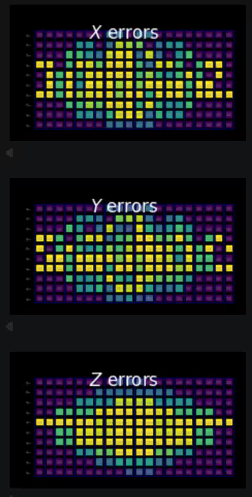
Each colored box in the output corresponds to a specific qubit at a specific time. The darkest (purple) boxes indicate a qubit and layer at which an error cannot propagate to the measurement(s) of interest. The brightest (yellow) boxes correspond to a qubit and layer at which an error can have a strong influence on the measurement(s) of interest.
Note the purple regions on the right of each map. An error at the same layer as the measurement, but on a different qubit, cannot affect the measurement through the circuit connectivity shown. Similarly, an error one layer back in time (one layer to the left) can only propagate to the adjacent qubit in the next step, because of the structure of the entangling layer, and so on. So the cone shape on the right is general whenever relatively few qubits are involved in the measurement of interest.
Check your understanding
Do you think it is better to make a shaded lightcone map before or after transpilation? Why?
Answer
It must be done after transpilation. In order for these different maps to be useful we must make sure that the adjacent qubits in our circuit corresponded to adjacent qubits on our quantum chip. Otherwise, entangling gates shown as acting on the adjacent qubits in the circuit diagram would end up requiring SWAP gates and a more complicated circuit structure.