Diagonalizzazione quantistica di Krylov di Hamiltoniane su reticolo

Stima di utilizzo: 70 minuti su un processore Heron o Nighthawk (NOTA: Questa è solo una stima. Il tuo tempo di esecuzione potrebbe variare.)

Risultati di apprendimento

• Come interpretare la diagonalizzazione quantistica di Krylov (KQD) come apprendimento di una funzione Hamiltoniana finita che agisce come filtro spettrale.

• Come costruire le matrici Hamiltoniana e di overlap proiettate con misurazioni di extended swap-test.

• Come risolvere il problema agli autovalori generalizzato (GEVP) risultante e recuperare una stima dell'energia dello stato fondamentale per una Hamiltoniana su reticolo.

Prerequisiti

• Primitive di Qiskit

• Stima dell'energia dello stato fondamentale della catena di Heisenberg con VQE

• Corso sugli algoritmi di diagonalizzazione quantistica

Contesto

Questo tutorial dimostra come implementare l'algoritmo di diagonalizzazione quantistica di Krylov (KQD) nel contesto dei pattern Qiskit. Imparerai prima la teoria alla base dell'algoritmo e poi vedrai una dimostrazione della sua esecuzione su una QPU.

Stimare le proprietà a bassa energia di Hamiltoniane a molti corpi è un compito centrale nella simulazione quantistica. Ad esempio, le energie dello stato fondamentale e le eccitazioni a bassa energia sono direttamente correlate alla stabilità chimica, all'ordinamento magnetico, alle transizioni di fase quantistiche e alla risposta dei materiali. Su un computer classico, la dimensione dello spazio di Hilbert cresce esponenzialmente con il numero di orbitali o spin, quindi la diagonalizzazione diretta diventa rapidamente impraticabile.

Esistono diversi approcci di calcolo quantistico a questo problema. I metodi variazionali a breve termine, come l'eigensolver variazionale quantistico (VQE), utilizzano circuiti parametrizzati relativamente poco profondi, ma richiedono un ciclo di ottimizzazione classica non lineare con molte valutazioni del circuito quantistico. All'altro estremo, la stima di fase quantistica (QPE) fornisce un percorso più diretto alla stima degli autovalori con garanzie rigorose, ma la QPE standard richiede circuiti coerenti lunghi ed è principalmente adatta a computer quantistici fault-tolerant. La KQD si colloca tra questi due approcci: utilizza l'evoluzione Hamiltoniana in tempo reale, come negli algoritmi basati sulla stima di fase, ma sostituisce la stima di fase completa con un problema agli autovalori proiettato compatto che può essere risolto classicamente.

Consideriamo un'Hamiltoniana a $n$ qubit $H$ e uno stato di riferimento $\lvert \psi_{0}\rangle$. Il metodo KQD costruisce un sottospazio di Krylov da stati evoluti in tempo reale,

$$\begin{equation*} \lvert \psi_\ell\rangle = e^{-i\ell\Delta t H}\lvert \psi_{0}\rangle, \qquad \ell = 0,1,\ldots,r-1, \end{equation*}$$

dove $r$ è la dimensione di Krylov e $\Delta t$ è il passo temporale. Qualsiasi stato nel sottospazio di Krylov è quindi rappresentato come una combinazione lineare di questi stati di base,

$$\begin{equation*} \lvert \psi(\mathbf{c})\rangle = \frac{\sum_{\ell=0}^{r-1} c_\ell \lvert \psi_\ell\rangle} {\left\|\sum_{\ell=0}^{r-1} c_\ell \lvert \psi_\ell\rangle\right\|}, \end{equation*}$$

where the denominator normalizes the state.

Con una semplice algebra, possiamo vedere che l'energia corrispondente è scritta come il quoziente di Rayleigh,

$$\begin{equation*} E(\mathbf{c}) =\langle \psi(\mathbf{c})|H|\psi(\mathbf{c}) \rangle= \frac{ \sum_{k,\ell} c_k^* c_\ell \langle \psi_k\vert H\vert\psi_\ell\rangle }{ \sum_{k,\ell} c_k^* c_\ell \langle \psi_k\vert\psi_\ell\rangle } = \frac{ \mathbf{c}^{\dagger}\mathcal{H}\mathbf{c} }{ \mathbf{c}^{\dagger}\mathcal{S}\mathbf{c} }. \end{equation*}$$

Qui, le matrici $\mathcal{S}$ e $\mathcal{H}$,

$$\begin{equation*} \mathcal{S}_{k\ell}=\langle \psi_k\vert\psi_\ell\rangle, \qquad \mathcal{H}_{k\ell}=\langle \psi_k\vert H\vert\psi_\ell\rangle \end{equation*}$$

definiscono le matrici di overlap e Hamiltoniana proiettate. I loro elementi sono stimati utilizzando misurazioni di circuiti quantistici.

Miriamo a trovare il coefficiente $\mathbf{c}$ che fornisce il minimo $E(\mathbf{c})$:

$$\begin{equation*} \min_{\mathbf{c}\neq \mathbf{0}} E(\mathbf{c}). \end{equation*}$$

Per il teorema di Rayleigh-Ritz, questa minimizzazione è equivalente a risolvere il problema agli autovalori generalizzato (GEVP),

$$\begin{equation*} \mathcal{H}\mathbf{c}=E \mathcal{S}\mathbf{c}. \end{equation*}$$

Nota che la dimensione $r$ può essere abbastanza piccola da permettere a un computer classico di risolvere il GEVP.

Questo è lo stesso principio variazionale utilizzato nella diagonalizzazione classica dei sottospazi, ma qui gli stati di base sono generati dall'evoluzione temporale quantistica. Rispetto al VQE, la KQD richiede solitamente circuiti più profondi perché si basa sull'evoluzione in tempo reale. In cambio, la KQD evita l'ottimizzazione non lineare dei parametri e l'esecuzione iterativa su hardware quantistico, e migliora sistematicamente man mano che il sottospazio proiettato viene ampliato. L'algoritmo è stato dimostrato su larga scala su hardware quantistico esistente [2], e le sue prestazioni possono essere analizzate con garanzie dimostrabili [1].

Requisiti

Prima di iniziare questo tutorial, assicuratevi di avere installato quanto segue:

• Qiskit SDK v2.3 o successivo con supporto per la visualizzazione

• Qiskit Runtime v0.22 o successivo ( pip install qiskit-ibm-runtime )

• SciPy (pip install scipy)

• Matplotlib (pip install matplotlib)

• Pandas (pip install pandas)

L'esecuzione sull'hardware richiede qiskit-ibm-runtime e l'accesso a un account IBM Quantum®.

Configurazione

La cella di setup importa i moduli richiesti e definisce le funzioni helper per il workflow:

1. costruire l'Hamiltoniana di Heisenberg;

2. risolvere il GEVP con soglia;

3. valutare il filtro di Krylov appreso;

4. convertire i valori del filtro in pesi spettrali;

5. tracciare le distribuzioni di energia di riferimento e filtrate.

# Added by doQumentation — installs the packages this notebook needs if they are missing
import importlib.util

_needed = {"matplotlib": "matplotlib", "numpy": "numpy", "pandas": "pandas", "qiskit": "qiskit", "qiskit_ibm_runtime": "qiskit-ibm-runtime", "scipy": "scipy"}
_missing = [pip for module, pip in _needed.items()
            if importlib.util.find_spec(module) is None]
# One at a time, so a package that fails to install does not block the others
for _pip in _missing:
    %pip install -q {_pip}
if not _missing:
    print("\u2713 All required packages are installed")

from __future__ import annotations

import warnings

import numpy as np
import pandas as pd
import scipy.linalg as la
import matplotlib.pyplot as plt

from qiskit import QuantumCircuit, transpile
from qiskit.circuit import Parameter
from qiskit.circuit.library import PauliEvolutionGate
from qiskit.primitives import StatevectorEstimator
from qiskit.quantum_info import Operator, SparsePauliOp
from qiskit.synthesis import LieTrotter, SuzukiTrotter
from qiskit.transpiler import PassManager, Layout
from qiskit.transpiler.passes import CommutativeOptimization
from qiskit.transpiler.preset_passmanagers import generate_preset_pass_manager
from qiskit_ibm_runtime import QiskitRuntimeService, EstimatorV2, Batch
from qiskit_ibm_runtime.fake_provider import FakeMarrakesh

warnings.filterwarnings("ignore")

def make_heisenberg_hamiltonian(
    num_qubits: int,
    coupling: float = 1.0,
) -> SparsePauliOp:
    """Make a Heisenberg Hamiltonian for a 1D chain of qubits with nearest-neighbor interactions."""
    terms: list[tuple[str, complex]] = []

    def append_term(q0: int, q1: int, pauli: str):
        label = ["I"] * num_qubits
        label[num_qubits - 1 - q0] = pauli[0]
        label[num_qubits - 1 - q1] = pauli[1]
        terms.append(("".join(label), coupling))

    for pauli in ("XX", "YY", "ZZ"):
        for q in range(num_qubits - 1):
            append_term(q, q + 1, pauli)
    return SparsePauliOp.from_list(terms).simplify()

def _basis_state_transition_amplitude_sparse(
    hamiltonian: SparsePauliOp,
    bra_state: int,
    ket_state: int,
) -> complex:
    """Evaluate <bra_state|H|ket_state> for computational-basis states."""
    num_qubits = hamiltonian.num_qubits
    amplitude = 0.0 + 0.0j
    for pauli, coeff in zip(hamiltonian.paulis, hamiltonian.coeffs):
        new_state = ket_state
        phase = 1.0 + 0.0j
        for q in range(num_qubits):
            x = bool(pauli.x[q])
            z = bool(pauli.z[q])
            if not x and not z:
                continue
            bit = (new_state >> q) & 1
            if x and z:
                # Y|0> = i|1>, Y|1> = -i|0>
                phase *= 1j if bit == 0 else -1j
                new_state ^= 1 << q
            elif x:
                new_state ^= 1 << q
            else:
                # Z|0> = |0>, Z|1> = -|1>
                if bit:
                    phase *= -1
        if new_state == bra_state:
            amplitude += coeff * phase
    return amplitude

def basis_state_expectation_sparse(
    hamiltonian: SparsePauliOp,
    bitstring: str,
) -> complex:
    """Evaluate <bitstring|H|bitstring>."""
    state = int(bitstring, 2)
    return _basis_state_transition_amplitude_sparse(
        hamiltonian,
        bra_state=state,
        ket_state=state,
    )

def diagonalize_single_1_subspace(
    hamiltonian: SparsePauliOp,
) -> np.ndarray:
    """Diagonalize the Hamiltonian projected onto the single-excitation subspace."""
    num_qubits = hamiltonian.num_qubits

    # Integer basis states |...010...>, with the excitation at qubit k.
    basis = [1 << k for k in range(num_qubits)]

    h_single = np.empty((num_qubits, num_qubits), dtype=complex)

    for row, bra_state in enumerate(basis):
        for col, ket_state in enumerate(basis):
            h_single[row, col] = _basis_state_transition_amplitude_sparse(
                hamiltonian,
                bra_state=bra_state,
                ket_state=ket_state,
            )
    # Remove floating-point-level asymmetry.
    h_single = 0.5 * (h_single + h_single.conj().T)
    evals, _ = np.linalg.eigh(h_single)
    return np.real(evals)

def simple_transpilation(circuit: QuantumCircuit) -> QuantumCircuit:
    """Transpilation to simplify the circuit"""
    pm = PassManager(
        [
            CommutativeOptimization(),
        ]
    )
    circuit = transpile(circuit, optimization_level=3)
    circuit = pm.run(circuit)
    return circuit

def summarize_circuit(circuit: QuantumCircuit) -> dict[str, int | str]:
    """Summarize the circuit with depth, size, and 2-qubit gate information."""
    two_qubit_total = sum(
        inst.operation.num_qubits == 2 for inst in circuit.data
    )
    two_qubit_depth = circuit.depth(lambda x: x[0].num_qubits == 2)
    return {
        "depth": circuit.depth(),
        "size": circuit.size(),
        "2q gates": two_qubit_total,
        "2q depth": two_qubit_depth,
    }

def solve_thresholded_gevp(
    h_matrix: np.ndarray,
    s_matrix: np.ndarray,
    threshold: float = 1e-10,
) -> tuple[float, np.ndarray, int]:
    """Solve H c = E S c using canonical orthogonalization of S."""
    s_vals, s_vecs = la.eigh(s_matrix)

    valid = s_vals > threshold
    if not np.any(valid):
        raise ValueError(
            "All overlap eigenvalues were removed by thresholding."
        )

    keep = valid

    orthogonalizer = s_vecs[:, keep] @ np.diag(1.0 / np.sqrt(s_vals[keep]))
    h_orth = orthogonalizer.conj().T @ h_matrix @ orthogonalizer
    h_orth = 0.5 * (h_orth + h_orth.conj().T)

    eigvals, eigvecs = la.eigh(h_orth)

    coeffs = orthogonalizer @ eigvecs[:, 0]
    normalization = np.sqrt(np.real(coeffs.conj().T @ s_matrix @ coeffs))
    coeffs /= normalization

    return float(np.real(eigvals[0])), coeffs, int(np.sum(keep))

Nella prima parte di questo tutorial, dimostriamo il metodo KQD utilizzando un simulatore locale di statevector. In seguito, utilizziamo un backend quantistico reale per affrontare un problema su scala utility.

Definiamo anche un backend fittizio per dimostrare la transpilazione specifica per backend e ispezionare il circuito risultante.

try:
    service = QiskitRuntimeService()
except Exception:
    QiskitRuntimeService.save_account(
        token="<api_token>", instance="<instance>", overwrite=True
    )
    service = QiskitRuntimeService()

backend = FakeMarrakesh()

Esempio di simulatore su piccola scala

Step 1: Mappare gli input classici a un problema quantistico

Hamiltoniana e stato di riferimento

Questo esempio utilizza una catena di Heisenberg a condizioni al contorno aperte con 12 qubit ($n=12$),

$$\begin{equation*} H=\sum_{i=0}^{n-2}\left(X_iX_{i+1}+Y_iY_{i+1}+Z_iZ_{i+1}\right), \end{equation*}$$

con uno stato prodotto a singola eccitazione

$$\begin{equation*} |\psi_{0}\rangle=|000001000000\rangle \end{equation*}$$

come stato di riferimento. Poiché l'Hamiltoniana di Heisenberg definita sopra conserva il numero totale di eccitazioni, lo stato di riferimento rimane nel sottospazio a singola eccitazione, la cui dimensione cresce solo linearmente con il numero di qubit. Possiamo quindi calcolare l'energia esatta dello stato fondamentale in modo efficiente, diagonalizzando l'Hamiltoniana ristretta a quel sottospazio, e utilizzarla puramente come benchmark diagnostico per la stima KQD. Il workflow KQD stesso stima gli elementi della matrice proiettata utilizzando le primitive di Qiskit e risolve classicamente il problema proiettato risultante.

# Problem definition for the simulator example
num_qubits = 12
hamiltonian = make_heisenberg_hamiltonian(num_qubits=num_qubits, coupling=1.0)
ref_bitstring = "000001000000"
ref_energy = basis_state_expectation_sparse(hamiltonian, ref_bitstring)

print("Hamiltonian:")
print(hamiltonian)
print(f"Reference state: |{ref_bitstring}>")
print("Reference energy: ", ref_energy)

Hamiltonian:
SparsePauliOp(['IIIIIIIIIIXX', 'IIIIIIIIIXXI', 'IIIIIIIIXXII', 'IIIIIIIXXIII', 'IIIIIIXXIIII', 'IIIIIXXIIIII', 'IIIIXXIIIIII', 'IIIXXIIIIIII', 'IIXXIIIIIIII', 'IXXIIIIIIIII', 'XXIIIIIIIIII', 'IIIIIIIIIIYY', 'IIIIIIIIIYYI', 'IIIIIIIIYYII', 'IIIIIIIYYIII', 'IIIIIIYYIIII', 'IIIIIYYIIIII', 'IIIIYYIIIIII', 'IIIYYIIIIIII', 'IIYYIIIIIIII', 'IYYIIIIIIIII', 'YYIIIIIIIIII', 'IIIIIIIIIIZZ', 'IIIIIIIIIZZI', 'IIIIIIIIZZII', 'IIIIIIIZZIII', 'IIIIIIZZIIII', 'IIIIIZZIIIII', 'IIIIZZIIIIII', 'IIIZZIIIIIII', 'IIZZIIIIIIII', 'IZZIIIIIIIII', 'ZZIIIIIIIIII'],
              coeffs=[1.+0.j, 1.+0.j, 1.+0.j, 1.+0.j, 1.+0.j, 1.+0.j, 1.+0.j, 1.+0.j, 1.+0.j,
 1.+0.j, 1.+0.j, 1.+0.j, 1.+0.j, 1.+0.j, 1.+0.j, 1.+0.j, 1.+0.j, 1.+0.j,
 1.+0.j, 1.+0.j, 1.+0.j, 1.+0.j, 1.+0.j, 1.+0.j, 1.+0.j, 1.+0.j, 1.+0.j,
 1.+0.j, 1.+0.j, 1.+0.j, 1.+0.j, 1.+0.j, 1.+0.j])
Reference state: |000001000000>
Reference energy:  (7+0j)

Impostare i parametri per l'algoritmo

Sulla base dei limiti superiori sulla norma dell'Hamiltoniana, il Rif. [1] suggerisce euristicamente il passo temporale $\Delta t$ come $\pi/\|H\|$. Poiché la norma spettrale $\|H\|$ è difficile da calcolare, utilizziamo invece il suo limite superiore:

$$\begin{equation*} \|H\| \le \sum_{i=0}^{n-2}\underbrace{\|X_i X_{i+1}+Y_{i} Y_{i+1}+Z_{i} Z_{i+1}\|}_{4 \times 4 \text{ matrix, easy to calculate the norm}} = 3(n-1). \end{equation*}$$

Impostiamo la dimensione di Krylov a $r=10$ e il numero di passi di Trotter per passo temporale a $5$: uno spazio di Krylov abbastanza grande da risolvere lo spettro a bassa energia mantenendo il circuito più profondo ($t_{\max}=(r-1)\Delta t$) sostenibile, e abbastanza passi di Trotter da mantenere piccolo l'errore di discretizzazione a quel circuito più profondo.

dt = np.pi / (3 * (num_qubits - 1))
print("dt in Krylov basis:  ", dt)

krylov_dim = 10
num_trotter_steps = 5

dt in Krylov basis:   0.09519977738150888

Costruire il circuito

Qui, costruiamo i circuiti per stimare gli elementi della matrice $\mathcal{H}_{k\ell}$ e $\mathcal{S}_{k\ell}$. Poiché tutte le potenze di $H$ commutano, abbiamo

$$\begin{equation*} \mathcal{H}_{k\ell} = \langle\psi_{0}|H e^{-i(\ell-k)\Delta tH}|\psi_{0}\rangle=\mathcal{H}_{0,\ell-k}, \qquad \mathcal{S}_{k\ell} = \langle\psi_{0}|e^{-i(\ell-k)\Delta tH}|\psi_{0}\rangle=\mathcal{S}_{0,\ell-k}. \end{equation*}$$

Such matrices where the elements depend on the index differences in this manner are called Toeplitz and can be reconstructed from first-row elements indexed by $d=\ell-k$.

Qui, presentiamo il circuito, chiamato extended-swap-test, che prepara

$$\begin{equation*} |\Phi_{0d}\rangle= \frac{|0\rangle|\psi_0\rangle+|1\rangle|\psi_d\rangle}{\sqrt{2}}, \end{equation*}$$

dove $|\psi_d\rangle=e^{-id\Delta tH}|\psi_{0}\rangle$.

Stato di riferimento

Prepariamo lo stato di riferimento $|\psi_0\rangle$.

qc_ref = QuantumCircuit(num_qubits)
for i, b in enumerate(reversed(ref_bitstring)):
    if b == "1":
        qc_ref.x(i)
display(qc_ref.draw("mpl", scale=0.5))

Evoluzione temporale

Realizza l'operatore di evoluzione temporale generato dall'Hamiltoniana, approssimato tramite una semplice Lie-Trotterizzazione.

t = Parameter("t")

evol_gate = PauliEvolutionGate(
    hamiltonian,
    time=t,
    synthesis=LieTrotter(reps=num_trotter_steps),
    label="U(t)",
)

# Synthesize U(t) first and then control the synthesized circuit.
# This makes the controlled structure visible in the circuit drawer.
evolution_circuit = QuantumCircuit(num_qubits, name="U(t)")
evolution_circuit.append(evol_gate, range(num_qubits))
evolution_circuit = simple_transpilation(evolution_circuit)

# Make a controlled version of the evolution circuit.
controlled_evolution_gate = evolution_circuit.to_gate(label="U(t)").control(
    1, label="C-U(t)"
)
display(
    evolution_circuit.assign_parameters({t: 1.5}).draw(
        "mpl", scale=0.5, fold=-1
    )
)

Circuito di extended swap test [3]

Il circuito prepara prima lo stato di riferimento sul registro di sistema mentre l'ancilla rimane in $|0\rangle$:

$$\begin{equation*} |0\rangle |0\rangle^{\otimes n} \longrightarrow |0\rangle |\psi_{0}\rangle . \end{equation*}$$

Quindi, applicando una porta di Hadamard all'ancilla si crea una sovrapposizione coerente di due rami:

$$\begin{equation*} |0\rangle |\psi_0\rangle \longrightarrow \frac{|0\rangle + |1\rangle}{\sqrt{2}} |\psi_0\rangle = \frac{|0\rangle|\psi_0\rangle + |1\rangle|\psi_0\rangle}{\sqrt{2}} . \end{equation*}$$

Infine, la porta di evoluzione temporale controllata applica:

$$\begin{equation*} U(t=d\Delta t) = e^{-id\Delta t H} \end{equation*}$$

solo quando l'ancilla è nel ramo $|1\rangle$. Pertanto,

$$\begin{equation*} \frac{|0\rangle|\psi_0\rangle + |1\rangle|\psi_0\rangle}{\sqrt{2}} \longrightarrow \frac{|0\rangle|\psi_0\rangle + |1\rangle U(d\Delta t)|\psi_0\rangle}{\sqrt{2}} . \end{equation*}$$

Nel prossimo blocco di codice, implementiamo:

$$\begin{equation*} |\Psi(t)\rangle = \frac{|0\rangle|\psi_0\rangle + |1\rangle U(t)|\psi_0\rangle}{\sqrt{2}}, \end{equation*}$$

che sarà assegnato come $t=d\Delta t$ per $d=1,\cdots r-1$ nella fase di esecuzione.

ancilla = 0
system_qubits = list(range(1, num_qubits + 1))

extended_swap_test = QuantumCircuit(num_qubits + 1)

# Append state preparation part
extended_swap_test = extended_swap_test.compose(qc_ref, system_qubits)

# Prepare the coherent branch label, (|0> + |1>) / sqrt(2).
extended_swap_test.h(ancilla)

# Apply U(t) only to the |1> branch of the ancilla.
extended_swap_test.append(
    controlled_evolution_gate, [ancilla] + system_qubits
)

# Decompose once more for visualization so that control bullets are visible.
display(extended_swap_test.draw("mpl", fold=-1))

Osservabili

Per qualsiasi osservabile hermitiana di sistema $O$, qui impostiamo le osservabili da calcolare:

$$\begin{equation*} z=\langle \psi_0|O|\psi_d\rangle . \end{equation*}$$

Questo perché $O=I$ fornisce l'elemento di overlap $\mathcal{S}_{0d}=\langle\psi_0|\psi_d\rangle$, mentre $O=H$ fornisce l'elemento Hamiltoniano $\mathcal{H}_{0d}=\langle\psi_0|H|\psi_d\rangle$.

Utilizzando $X=|0\rangle\langle 1|+|1\rangle\langle 0|$, abbiamo

$$\begin{align*} \langle \Psi_{0d}|X\otimes O| \Psi_{0d} \rangle &= \left(\frac{\langle0|\langle\psi_0| + \langle1| \langle\psi_d|}{\sqrt{2}}\right)(X\otimes O)\left(\frac{|0\rangle|\psi_0\rangle + |1\rangle |\psi_d\rangle}{\sqrt{2}}\right) \\ &= \frac{1}{2} \left( \langle \psi_0|O|\psi_d\rangle + \langle \psi_d|O|\psi_0\rangle \right) \\ &= \frac{z+z^*}{2} = \operatorname{Re} z. \end{align*}$$

Analogamente, utilizzando $Y=-i|0\rangle\langle 1|+i|1\rangle\langle 0|$,

$$\begin{align*} \langle \Psi_{0d}|Y\otimes O| \Psi_{0d} \rangle &= \left(\frac{\langle0|\langle\psi_0| + \langle1| \langle\psi_d|}{\sqrt{2}}\right)(Y\otimes O)\left(\frac{|0\rangle|\psi_0\rangle + |1\rangle |\psi_d\rangle}{\sqrt{2}}\right) \\ &= \frac{1}{2} \left( -i\langle \psi_0|O|\psi_d\rangle + i\langle \psi_d|O|\psi_0\rangle \right) \\ &= \frac{-iz+iz^*}{2} = \operatorname{Im} z. \end{align*}$$

Pertanto, abbiamo

$$\begin{equation*} \langle \Phi_{0d}|X\otimes O|\Phi_{0d}\rangle = \operatorname{Re}\langle\psi_0|O|\psi_d\rangle , \quad \langle \Phi_{0d}|Y\otimes O|\Phi_{0d}\rangle = \operatorname{Im}\langle\psi_0|O|\psi_d\rangle . \end{equation*}$$

Infine, per ciascuno stato $|\Psi_{0d}\rangle$, dobbiamo misurare:

$$\begin{align*} X \otimes I \text{ for } \operatorname{Re}\mathcal{S}_{0d},\\ Y \otimes I \text{ for } \operatorname{Im}\mathcal{S}_{0d},\\ X \otimes H \text{ for } \operatorname{Re}\mathcal{H}_{0d},\\ Y \otimes H \text{ for } \operatorname{Im}\mathcal{H}_{0d}.\\ \end{align*}$$

n_qubits = hamiltonian.num_qubits

observable_labels = [
    "Re S_0d",
    "Im S_0d",
    "Re H_0d",
    "Im H_0d",
]

# X ⊗ I and Y ⊗ I.
# Qiskit's Pauli-label convention places qubit 0 on the rightmost character,
# so the ancilla Pauli is appended to the right.
obs_x_identity = SparsePauliOp("I" * n_qubits + "X")
obs_y_identity = SparsePauliOp("I" * n_qubits + "Y")

# X ⊗ H and Y ⊗ H.
obs_x_hamiltonian = SparsePauliOp.from_list(
    [
        (label + "X", coeff)
        for label, coeff in zip(
            hamiltonian.paulis.to_labels(),
            hamiltonian.coeffs,
        )
    ]
)

obs_y_hamiltonian = SparsePauliOp.from_list(
    [
        (label + "Y", coeff)
        for label, coeff in zip(
            hamiltonian.paulis.to_labels(),
            hamiltonian.coeffs,
        )
    ]
)

observables = [
    obs_x_identity,
    obs_y_identity,
    obs_x_hamiltonian,
    obs_y_hamiltonian,
]

for obs, label in zip(observables, observable_labels):
    print(f"Observable: {label}")
    print(obs)
    print()

Observable: Re S_0d
SparsePauliOp(['IIIIIIIIIIIIX'],
              coeffs=[1.+0.j])

Observable: Im S_0d
SparsePauliOp(['IIIIIIIIIIIIY'],
              coeffs=[1.+0.j])

Observable: Re H_0d
SparsePauliOp(['IIIIIIIIIIXXX', 'IIIIIIIIIXXIX', 'IIIIIIIIXXIIX', 'IIIIIIIXXIIIX', 'IIIIIIXXIIIIX', 'IIIIIXXIIIIIX', 'IIIIXXIIIIIIX', 'IIIXXIIIIIIIX', 'IIXXIIIIIIIIX', 'IXXIIIIIIIIIX', 'XXIIIIIIIIIIX', 'IIIIIIIIIIYYX', 'IIIIIIIIIYYIX', 'IIIIIIIIYYIIX', 'IIIIIIIYYIIIX', 'IIIIIIYYIIIIX', 'IIIIIYYIIIIIX', 'IIIIYYIIIIIIX', 'IIIYYIIIIIIIX', 'IIYYIIIIIIIIX', 'IYYIIIIIIIIIX', 'YYIIIIIIIIIIX', 'IIIIIIIIIIZZX', 'IIIIIIIIIZZIX', 'IIIIIIIIZZIIX', 'IIIIIIIZZIIIX', 'IIIIIIZZIIIIX', 'IIIIIZZIIIIIX', 'IIIIZZIIIIIIX', 'IIIZZIIIIIIIX', 'IIZZIIIIIIIIX', 'IZZIIIIIIIIIX', 'ZZIIIIIIIIIIX'],
              coeffs=[1.+0.j, 1.+0.j, 1.+0.j, 1.+0.j, 1.+0.j, 1.+0.j, 1.+0.j, 1.+0.j, 1.+0.j,
 1.+0.j, 1.+0.j, 1.+0.j, 1.+0.j, 1.+0.j, 1.+0.j, 1.+0.j, 1.+0.j, 1.+0.j,
 1.+0.j, 1.+0.j, 1.+0.j, 1.+0.j, 1.+0.j, 1.+0.j, 1.+0.j, 1.+0.j, 1.+0.j,
 1.+0.j, 1.+0.j, 1.+0.j, 1.+0.j, 1.+0.j, 1.+0.j])

Observable: Im H_0d
SparsePauliOp(['IIIIIIIIIIXXY', 'IIIIIIIIIXXIY', 'IIIIIIIIXXIIY', 'IIIIIIIXXIIIY', 'IIIIIIXXIIIIY', 'IIIIIXXIIIIIY', 'IIIIXXIIIIIIY', 'IIIXXIIIIIIIY', 'IIXXIIIIIIIIY', 'IXXIIIIIIIIIY', 'XXIIIIIIIIIIY', 'IIIIIIIIIIYYY', 'IIIIIIIIIYYIY', 'IIIIIIIIYYIIY', 'IIIIIIIYYIIIY', 'IIIIIIYYIIIIY', 'IIIIIYYIIIIIY', 'IIIIYYIIIIIIY', 'IIIYYIIIIIIIY', 'IIYYIIIIIIIIY', 'IYYIIIIIIIIIY', 'YYIIIIIIIIIIY', 'IIIIIIIIIIZZY', 'IIIIIIIIIZZIY', 'IIIIIIIIZZIIY', 'IIIIIIIZZIIIY', 'IIIIIIZZIIIIY', 'IIIIIZZIIIIIY', 'IIIIZZIIIIIIY', 'IIIZZIIIIIIIY', 'IIZZIIIIIIIIY', 'IZZIIIIIIIIIY', 'ZZIIIIIIIIIIY'],
              coeffs=[1.+0.j, 1.+0.j, 1.+0.j, 1.+0.j, 1.+0.j, 1.+0.j, 1.+0.j, 1.+0.j, 1.+0.j,
 1.+0.j, 1.+0.j, 1.+0.j, 1.+0.j, 1.+0.j, 1.+0.j, 1.+0.j, 1.+0.j, 1.+0.j,
 1.+0.j, 1.+0.j, 1.+0.j, 1.+0.j, 1.+0.j, 1.+0.j, 1.+0.j, 1.+0.j, 1.+0.j,
 1.+0.j, 1.+0.j, 1.+0.j, 1.+0.j, 1.+0.j, 1.+0.j])

Per la stima degli elementi della matrice $\mathcal{H}$, il numero di termini di Pauli è molto maggiore rispetto a quello per gli elementi della matrice $\mathcal{S}$.

Possiamo ora ridurre il numero di termini Hamiltoniani misurati utilizzando una tecnica di shifting [4]. Dividiamo l'Hamiltoniana come:

$$\begin{equation*} H = (H-T) + T, \end{equation*}$$

dove $T$ è scelto in modo tale che lo stato di riferimento sia il suo autostato,

$$\begin{equation*} T|\psi_0\rangle = \tau |\psi_0\rangle . \end{equation*}$$

Then,

$$\begin{align*} \mathcal{H}_{0d} &= \langle\psi_0|H|\psi_d\rangle \\ &= \langle\psi_0|(H-T)|\psi_d\rangle + \langle\psi_0|T|\psi_d\rangle \\ &= \langle\psi_0|(H-T)|\psi_d\rangle + \tau \langle\psi_0|\psi_d\rangle \\ &= \widetilde{\mathcal{H}}_{0d} + \tau \mathcal{S}_{0d}. \end{align*}$$

Here,

$$\begin{equation*} \widetilde{\mathcal{H}}_{0d} = \langle\psi_0|(H-T)|\psi_d\rangle \end{equation*}$$

è l'elemento della matrice Hamiltoniana shiftata. Pertanto, dobbiamo misurare solo $X\otimes (H-T)$ e $Y\otimes (H-T)$. Il contributo di $T$ viene ricostruito classicamente utilizzando l'elemento della matrice di overlap $\mathcal{S}_{0d}$ già misurato.

In questo esempio, una scelta naturale è la parte diagonale dell'Hamiltoniana di Heisenberg,

$$\begin{equation*} T = \sum_{i=0}^{n-2} Z_iZ_{i+1}. \end{equation*}$$

Poiché lo stato di riferimento è uno stato della base computazionale, è un autostato di ogni termine $Z_iZ_{i+1}$.

Tuttavia, una scelta più vantaggiosa è includere non solo i termini diagonali $ZZ$, ma anche i termini $XX+YY$ che annichilano lo stato di riferimento.

Per ogni coppia vicina, l'operatore $XX+YY$ soddisfa

$$\begin{equation*} (XX+YY)|00\rangle = 0, \qquad (XX+YY)|11\rangle = 0, \end{equation*}$$

and

$$\begin{equation*} (XX+YY)|01\rangle = 2|10\rangle, \qquad (XX+YY)|10\rangle = 2|01\rangle . \end{equation*}$$

Pertanto, il termine $XX+YY$ contribuisce solo quando i due qubit vicini hanno occupazioni diverse nella stringa binaria di riferimento. Se entrambi i qubit sono $0$ o entrambi $1$, il termine annichila lo stato di riferimento e può anch'esso essere shiftato fuori.

Sia $|\psi_{\rm ref}\rangle = |z_0\cdots z_{n-1}\rangle$, dove $z_i \in \{0,1\}$. Quindi, possiamo scegliere

$$\begin{equation*} T=\sum_{i=0}^{n-2} Z_iZ_{i+1} + \sum_{z_i={z_{i+1}}} \left( X_iX_{i+1} + Y_iY_{i+1} \right). \end{equation*}$$

Questo operatore soddisfa ancora

$$\begin{equation*} T|\psi_0\rangle = \tau |\psi_0\rangle , \end{equation*}$$

perché i termini $ZZ$ agiscono diagonalmente su $|\psi_0\rangle$, mentre i termini shiftati $XX+YY$ danno zero. L'autovalore corrispondente è quindi determinato solo dai termini $ZZ$,

$$\begin{equation*} \tau = \sum_{i=0}^{n-2} (-1)^{z_i} (-1)^{z_{i+1}} . \end{equation*}$$

Con questa scelta, l'Hamiltoniana shiftata diventa:

$$\begin{equation*} H-T = \sum_{z_i\ne z_{i+1}} \left( X_iX_{i+1} + Y_iY_{i+1} \right). \end{equation*}$$

Di conseguenza, è necessario misurare solo gli archi con occupazioni diverse nello stato di riferimento. Tutti i termini $ZZ$ e tutti i termini $XX+YY$ inattivi sono ricostruiti tramite il contributo di overlap $\tau \mathcal{S}_{0d}$, oppure danno contributo zero per costruzione.

Questo fornisce un'osservabile più piccola rispetto allo shifting solo della parte diagonale. In particolare, per uno stato di riferimento della base computazionale con un'eccitazione localizzata, solo gli archi adiacenti all'eccitazione rimangono in $H-T$. Pertanto, il numero di termini di Pauli in $X\otimes(H-T)$ e $Y\otimes(H-T)$ può essere sostanzialmente ridotto, mentre l'elemento di matrice ricostruito

$$\begin{equation*} \widetilde{\mathcal{H}}_{0d} + \tau \mathcal{S}_{0d} \end{equation*}$$

rimane esattamente lo stesso.

def make_reduced_heisenberg_observables(
    ref_bitstring: str,
    coupling: float = 1.0,
) -> tuple[SparsePauliOp, SparsePauliOp, float]:
    """Build X⊗(H-T), Y⊗(H-T), and tau."""
    n_qubits = len(ref_bitstring)

    shifted_terms: list[tuple[str, complex]] = []
    tau = 0.0

    def bit(q: int) -> str:
        return ref_bitstring[n_qubits - 1 - q]

    def append_term(q0: int, q1: int, pauli: str):
        label = ["I"] * n_qubits
        label[n_qubits - 1 - q0] = pauli[0]
        label[n_qubits - 1 - q1] = pauli[1]
        shifted_terms.append(("".join(label), coupling))

    for q in range(n_qubits - 1):
        same_occupation = bit(q) == bit(q + 1)

        # ZZ contribution to tau
        tau += coupling * (1.0 if same_occupation else -1.0)

        # XX + YY survives only for opposite occupations.
        if not same_occupation:
            append_term(q, q + 1, "XX")
            append_term(q, q + 1, "YY")

    if shifted_terms:
        obs_x_shifted_hamiltonian = SparsePauliOp.from_list(
            [(label + "X", coeff) for label, coeff in shifted_terms]
        )
        obs_y_shifted_hamiltonian = SparsePauliOp.from_list(
            [(label + "Y", coeff) for label, coeff in shifted_terms]
        )
    else:
        obs_x_shifted_hamiltonian = SparsePauliOp(
            "I" * n_qubits + "X", coeffs=[0.0]
        )
        obs_y_shifted_hamiltonian = SparsePauliOp(
            "I" * n_qubits + "Y", coeffs=[0.0]
        )

    return obs_x_shifted_hamiltonian, obs_y_shifted_hamiltonian, tau

obs_x_shifted_hamiltonian, obs_y_shifted_hamiltonian, shift_tau = (
    make_reduced_heisenberg_observables(ref_bitstring)
)

print("Observable: Re shifted H_0d")
print(obs_x_shifted_hamiltonian)
print()

print("Observable: Im shifted H_0d")
print(obs_y_shifted_hamiltonian)
print()

print("tau =", shift_tau)

observables = [
    obs_x_identity,
    obs_y_identity,
    obs_x_shifted_hamiltonian,
    obs_y_shifted_hamiltonian,
]
observable_labels = [
    "Re S_0d",
    "Im S_0d",
    "Re shifted H_0d",
    "Im shifted H_0d",
]

Observable: Re shifted H_0d
SparsePauliOp(['IIIIIXXIIIIIX', 'IIIIIYYIIIIIX', 'IIIIXXIIIIIIX', 'IIIIYYIIIIIIX'],
              coeffs=[1.+0.j, 1.+0.j, 1.+0.j, 1.+0.j])

Observable: Im shifted H_0d
SparsePauliOp(['IIIIIXXIIIIIY', 'IIIIIYYIIIIIY', 'IIIIXXIIIIIIY', 'IIIIYYIIIIIIY'],
              coeffs=[1.+0.j, 1.+0.j, 1.+0.j, 1.+0.j])

tau = 7.0

Step 2: Ottimizzare il problema per l'esecuzione su hardware quantistico

Ora trasformiamo il circuito astratto di extended-swap-test in un template orientato all'hardware. Prima di ciò, ottimizziamo ulteriormente il circuito a livello astratto.

Confrontare l'ordinamento dei termini Hamiltoniani

Innanzitutto, confrontiamo diversi ordinamenti dei termini di Pauli nell'Hamiltoniana di Heisenberg per la simulazione Hamiltoniana. L'Hamiltoniana stessa rimane invariata, ma l'ordinamento influisce sul modo in cui viene generato il circuito a formula prodotto e su quanto la struttura può essere parallelizzata nel circuito. Ad esempio, l'ordinamento ingenuo elenca tutti i termini $XX$ tra primi vicini, poi tutti i termini $YY$, poi tutti i termini $ZZ$. Questo pone archi adiacenti come $(0,1)$ e $(1,2)$ vicini tra loro, quindi non possono essere eseguiti in parallelo. L'ordinamento pari-poi-dispari visita prima gli archi pari disgiunti, seguiti dagli archi dispari, il che espone livelli paralleli a due qubit. L'ordinamento raggruppato per archi pari-dispari va un passo oltre: per ogni arco, mantiene insieme i termini locali $XX$, $YY$ e $ZZ$, pur visitando ancora gli archi pari prima di quelli dispari. Ci aspettiamo che gli ordinamenti pari-poi-dispari e raggruppato per archi pari-dispari riducano la profondità del circuito esponendo livelli paralleli a due qubit, e che l'ordinamento raggruppato per archi riduca inoltre l'errore di Trotter perché l'interazione locale a due qubit sullo stesso arco viene gestita come un blocco compatto.

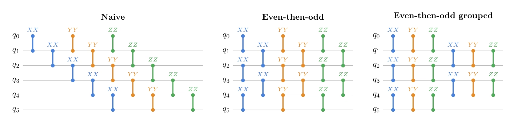
L'ordinamento Hamiltoniano influisce anche sull'errore di Trotter. Se poniamo termini non commutanti vicini tra loro, le transizioni di base si verificano più spesso, il che induce più errore di Trotter. Raggruppando i termini che richiedono la stessa trasformazione della base di Pauli, si possono evitare cambi di base ridondanti.

Qui, il confronto utilizza il tempo di evoluzione più grande che compare nelle stime di Krylov della prima riga, $t_{\max} = (r-1)\Delta t,$ utilizzando la stessa condizione di transpilazione.

Per misurare l'errore di Trotter, utilizziamo l'infedeltà di processo tra il circuito Trotterizzato e l'evoluzione Hamiltoniana esatta,

$$\begin{equation*} \text{Infidelity}(U,V) = 1-F(U,V) = 1 - \frac{|\operatorname{Tr}(U^\dagger V)|^2}{d^2}, \end{equation*}$$

where $d=2^n$ is the dimension of the Hilbert space.

Questa diagnostica utilizza matrici dense, quindi è adatta a questo piccolo esempio a 12 qubit ma non è pensata come subroutine scalabile.

# The comparison uses the largest time that appears in the first-row Krylov estimates.
# Circuit depth does not depend on this numeric value, but the Trotter error does.
comparison_time = (krylov_dim - 1) * dt

def make_heisenberg_hamiltonian_ordered(
    num_qubits: int,
    ordering: str,
    coupling: float = 1.0,
) -> SparsePauliOp:
    """Return the same Heisenberg Hamiltonian with a specified term ordering."""
    terms: list[tuple[str, complex]] = []
    even_edges = [(q, q + 1) for q in range(0, num_qubits - 1, 2)]
    odd_edges = [(q, q + 1) for q in range(1, num_qubits - 1, 2)]

    def append_term(q0: int, q1: int, pauli: str):
        label = ["I"] * num_qubits
        label[num_qubits - 1 - q0] = pauli[0]
        label[num_qubits - 1 - q1] = pauli[1]
        terms.append(("".join(label), coupling))

    if ordering == "naive":
        for pauli in ("XX", "YY", "ZZ"):
            for q in range(num_qubits - 1):
                append_term(q, q + 1, pauli)
    elif ordering == "even-then-odd":
        for pauli in ("XX", "YY", "ZZ"):
            for q0, q1 in even_edges + odd_edges:
                append_term(q0, q1, pauli)
    elif ordering == "even-odd edge-grouped":
        for q0, q1 in even_edges + odd_edges:
            for pauli in ("XX", "YY", "ZZ"):
                append_term(q0, q1, pauli)
    else:
        raise ValueError(f"Unknown ordering: {ordering}")

    return SparsePauliOp.from_list(terms).simplify()

def build_numeric_evolution_circuit(
    hamiltonian: SparsePauliOp,
    synthesis,
    time_value: float,
    **synthesis_kwargs,
) -> QuantumCircuit:
    """Build a numeric circuit for exp(-i H t) with a chosen synthesis rule."""
    evolution_gate = PauliEvolutionGate(
        hamiltonian,
        time=time_value,
        synthesis=synthesis(**synthesis_kwargs),
    )
    circuit = QuantumCircuit(hamiltonian.num_qubits)
    circuit.append(evolution_gate, range(hamiltonian.num_qubits))
    return circuit

def process_infidelity(
    circuit: QuantumCircuit,
    exact_matrix: np.ndarray,
) -> float:
    """Return 1 - |Tr(U_circuit† U_exact) / d|²."""
    circuit_matrix = np.asarray(Operator(circuit).data)
    dim = circuit_matrix.shape[0]
    normalized_trace = np.vdot(circuit_matrix, exact_matrix) / dim
    fidelity = np.abs(normalized_trace) ** 2
    return float(np.clip(1.0 - fidelity, 0.0, 1.0))

hamiltonians_by_ordering = {
    ordering: make_heisenberg_hamiltonian_ordered(
        num_qubits, ordering, coupling=1.0
    )
    for ordering in ["naive", "even-then-odd", "even-odd edge-grouped"]
}

print(f"Comparison time: {comparison_time}\n")

for order_name, ham_ordered in hamiltonians_by_ordering.items():
    print(f"{order_name}:")
    print([op for op, _ in ham_ordered.to_list()])
    print()

print("Precomputing the exact evolution operator... ", end="")
exact_matrix = la.expm(-1j * comparison_time * hamiltonian.to_matrix())
print("Done")

Comparison time: 0.8567979964335799

naive:
['IIIIIIIIIIXX', 'IIIIIIIIIXXI', 'IIIIIIIIXXII', 'IIIIIIIXXIII', 'IIIIIIXXIIII', 'IIIIIXXIIIII', 'IIIIXXIIIIII', 'IIIXXIIIIIII', 'IIXXIIIIIIII', 'IXXIIIIIIIII', 'XXIIIIIIIIII', 'IIIIIIIIIIYY', 'IIIIIIIIIYYI', 'IIIIIIIIYYII', 'IIIIIIIYYIII', 'IIIIIIYYIIII', 'IIIIIYYIIIII', 'IIIIYYIIIIII', 'IIIYYIIIIIII', 'IIYYIIIIIIII', 'IYYIIIIIIIII', 'YYIIIIIIIIII', 'IIIIIIIIIIZZ', 'IIIIIIIIIZZI', 'IIIIIIIIZZII', 'IIIIIIIZZIII', 'IIIIIIZZIIII', 'IIIIIZZIIIII', 'IIIIZZIIIIII', 'IIIZZIIIIIII', 'IIZZIIIIIIII', 'IZZIIIIIIIII', 'ZZIIIIIIIIII']

even-then-odd:
['IIIIIIIIIIXX', 'IIIIIIIIXXII', 'IIIIIIXXIIII', 'IIIIXXIIIIII', 'IIXXIIIIIIII', 'XXIIIIIIIIII', 'IIIIIIIIIXXI', 'IIIIIIIXXIII', 'IIIIIXXIIIII', 'IIIXXIIIIIII', 'IXXIIIIIIIII', 'IIIIIIIIIIYY', 'IIIIIIIIYYII', 'IIIIIIYYIIII', 'IIIIYYIIIIII', 'IIYYIIIIIIII', 'YYIIIIIIIIII', 'IIIIIIIIIYYI', 'IIIIIIIYYIII', 'IIIIIYYIIIII', 'IIIYYIIIIIII', 'IYYIIIIIIIII', 'IIIIIIIIIIZZ', 'IIIIIIIIZZII', 'IIIIIIZZIIII', 'IIIIZZIIIIII', 'IIZZIIIIIIII', 'ZZIIIIIIIIII', 'IIIIIIIIIZZI', 'IIIIIIIZZIII', 'IIIIIZZIIIII', 'IIIZZIIIIIII', 'IZZIIIIIIIII']

even-odd edge-grouped:
['IIIIIIIIIIXX', 'IIIIIIIIIIYY', 'IIIIIIIIIIZZ', 'IIIIIIIIXXII', 'IIIIIIIIYYII', 'IIIIIIIIZZII', 'IIIIIIXXIIII', 'IIIIIIYYIIII', 'IIIIIIZZIIII', 'IIIIXXIIIIII', 'IIIIYYIIIIII', 'IIIIZZIIIIII', 'IIXXIIIIIIII', 'IIYYIIIIIIII', 'IIZZIIIIIIII', 'XXIIIIIIIIII', 'YYIIIIIIIIII', 'ZZIIIIIIIIII', 'IIIIIIIIIXXI', 'IIIIIIIIIYYI', 'IIIIIIIIIZZI', 'IIIIIIIXXIII', 'IIIIIIIYYIII', 'IIIIIIIZZIII', 'IIIIIXXIIIII', 'IIIIIYYIIIII', 'IIIIIZZIIIII', 'IIIXXIIIIIII', 'IIIYYIIIIIII', 'IIIZZIIIIIII', 'IXXIIIIIIIII', 'IYYIIIIIIIII', 'IZZIIIIIIIII']

Precomputing the exact evolution operator... Done

Manteniamo prima fissa la regola di sintesi a un passo di Trotter del primo ordine e variamo solo l'ordinamento dei termini di Pauli. L'obiettivo di questo confronto è principalmente vedere quanto la profondità del circuito e il costo a due qubit possano essere ridotti esponendo al transpiler archi disgiunti tra primi vicini.

ordering_comparison_rows = []
infidelity_reps = [1, 2, 4, 8]

for ordering, ham_ordered in hamiltonians_by_ordering.items():
    for reps in infidelity_reps:
        circuit = build_numeric_evolution_circuit(
            ham_ordered,
            LieTrotter,
            comparison_time,
            reps=reps,
        )
        decomposed_circuit = simple_transpilation(circuit)
        infidelity = process_infidelity(decomposed_circuit, exact_matrix)
        ordering_comparison_rows.append(
            {
                "ordering": ordering,
                "synthesis": f"LieTrotter(reps={reps})",
                "infidelity": infidelity,
                **summarize_circuit(decomposed_circuit),
            }
        )
        if reps == 1:
            print(f"Circuit for {ordering} ordering:")
            print([op for op, _ in ham_ordered.to_list()])
            display(decomposed_circuit.draw("mpl", fold=-1, scale=0.6))

ordering_comparison_df = pd.DataFrame(ordering_comparison_rows)
display(ordering_comparison_df)

hamiltonian_for_synthesis = hamiltonians_by_ordering["even-odd edge-grouped"]

Circuit for naive ordering:
['IIIIIIIIIIXX', 'IIIIIIIIIXXI', 'IIIIIIIIXXII', 'IIIIIIIXXIII', 'IIIIIIXXIIII', 'IIIIIXXIIIII', 'IIIIXXIIIIII', 'IIIXXIIIIIII', 'IIXXIIIIIIII', 'IXXIIIIIIIII', 'XXIIIIIIIIII', 'IIIIIIIIIIYY', 'IIIIIIIIIYYI', 'IIIIIIIIYYII', 'IIIIIIIYYIII', 'IIIIIIYYIIII', 'IIIIIYYIIIII', 'IIIIYYIIIIII', 'IIIYYIIIIIII', 'IIYYIIIIIIII', 'IYYIIIIIIIII', 'YYIIIIIIIIII', 'IIIIIIIIIIZZ', 'IIIIIIIIIZZI', 'IIIIIIIIZZII', 'IIIIIIIZZIII', 'IIIIIIZZIIII', 'IIIIIZZIIIII', 'IIIIZZIIIIII', 'IIIZZIIIIIII', 'IIZZIIIIIIII', 'IZZIIIIIIIII', 'ZZIIIIIIIIII']

Circuit for even-then-odd ordering:
['IIIIIIIIIIXX', 'IIIIIIIIXXII', 'IIIIIIXXIIII', 'IIIIXXIIIIII', 'IIXXIIIIIIII', 'XXIIIIIIIIII', 'IIIIIIIIIXXI', 'IIIIIIIXXIII', 'IIIIIXXIIIII', 'IIIXXIIIIIII', 'IXXIIIIIIIII', 'IIIIIIIIIIYY', 'IIIIIIIIYYII', 'IIIIIIYYIIII', 'IIIIYYIIIIII', 'IIYYIIIIIIII', 'YYIIIIIIIIII', 'IIIIIIIIIYYI', 'IIIIIIIYYIII', 'IIIIIYYIIIII', 'IIIYYIIIIIII', 'IYYIIIIIIIII', 'IIIIIIIIIIZZ', 'IIIIIIIIZZII', 'IIIIIIZZIIII', 'IIIIZZIIIIII', 'IIZZIIIIIIII', 'ZZIIIIIIIIII', 'IIIIIIIIIZZI', 'IIIIIIIZZIII', 'IIIIIZZIIIII', 'IIIZZIIIIIII', 'IZZIIIIIIIII']

Circuit for even-odd edge-grouped ordering:
['IIIIIIIIIIXX', 'IIIIIIIIIIYY', 'IIIIIIIIIIZZ', 'IIIIIIIIXXII', 'IIIIIIIIYYII', 'IIIIIIIIZZII', 'IIIIIIXXIIII', 'IIIIIIYYIIII', 'IIIIIIZZIIII', 'IIIIXXIIIIII', 'IIIIYYIIIIII', 'IIIIZZIIIIII', 'IIXXIIIIIIII', 'IIYYIIIIIIII', 'IIZZIIIIIIII', 'XXIIIIIIIIII', 'YYIIIIIIIIII', 'ZZIIIIIIIIII', 'IIIIIIIIIXXI', 'IIIIIIIIIYYI', 'IIIIIIIIIZZI', 'IIIIIIIXXIII', 'IIIIIIIYYIII', 'IIIIIIIZZIII', 'IIIIIXXIIIII', 'IIIIIYYIIIII', 'IIIIIZZIIIII', 'IIIXXIIIIIII', 'IIIYYIIIIIII', 'IIIZZIIIIIII', 'IXXIIIIIIIII', 'IYYIIIIIIIII', 'IZZIIIIIIIII']

ordering           synthesis  infidelity  depth  size  \
0                   naive  LieTrotter(reps=1)    0.999917     15    33   
1                   naive  LieTrotter(reps=2)    0.805998     21    66   
2                   naive  LieTrotter(reps=4)    0.271389     33   132   
3                   naive  LieTrotter(reps=8)    0.074590     57   264   
4           even-then-odd  LieTrotter(reps=1)    0.999917      6    33   
5           even-then-odd  LieTrotter(reps=2)    0.805998     12    66   
6           even-then-odd  LieTrotter(reps=4)    0.271389     24   132   
7           even-then-odd  LieTrotter(reps=8)    0.074590     48   264   
8   even-odd edge-grouped  LieTrotter(reps=1)    0.998432      6    33   
9   even-odd edge-grouped  LieTrotter(reps=2)    0.653843     12    66   
10  even-odd edge-grouped  LieTrotter(reps=4)    0.181529     24   132   
11  even-odd edge-grouped  LieTrotter(reps=8)    0.045244     48   264   

    2q gates  2q depth  
0         33        15  
1         66        21  
2        132        33  
3        264        57  
4         33         6  
5         66        12  
6        132        24  
7        264        48  
8         33         6  
9         66        12  
10       132        24  
11       264        48

A reps=1, osserviamo che gli ordinamenti pari-poi-dispari e raggruppato per archi pari-dispari collassano entrambi la profondità da 15 a 6 esponendo livelli paralleli a due qubit, mentre il conteggio delle porte a due qubit rimane lo stesso in tutti e tre gli ordinamenti. Tuttavia, tutti e tre gli ordinamenti hanno un'infedeltà vicina a 1, quindi effettuiamo uno sweep del numero di ripetizioni di Trotter per separare più chiaramente gli ordinamenti. All'aumentare del numero di ripetizioni, l'infedeltà dell'ordinamento even-odd edge-grouped scende più rapidamente degli altri due, raggiungendo 0,045 a reps=8 contro 0,075 per l'ordinamento ingenuo e pari-poi-dispari.

Confrontare la sintesi a formula prodotto

Successivamente, esploriamo diverse impostazioni avanzate della Trotterizzazione, con l'ordinamento Hamiltoniano fisso all'ordinamento raggruppato per archi pari-dispari. Consideriamo Lie-Trotter del primo ordine, Suzuki-Trotter del secondo ordine e Suzuki-Trotter del quarto ordine.

synthesis_comparison_rows = []

for num_trotter_steps in [1, 2, 3, 4, 5]:
    synthesis_cases = [
        ("LieTrotter", LieTrotter, {"reps": num_trotter_steps}),
        (
            "SuzukiTrotter(order=2)",
            SuzukiTrotter,
            {"order": 2, "reps": num_trotter_steps},
        ),
        (
            "SuzukiTrotter(order=4)",
            SuzukiTrotter,
            {"order": 4, "reps": num_trotter_steps},
        ),
    ]
    for label, synthesis, kwargs in synthesis_cases:
        circuit = build_numeric_evolution_circuit(
            hamiltonian_for_synthesis,
            synthesis,
            comparison_time,
            **kwargs,
        )
        decomposed_circuit = simple_transpilation(circuit)
        synthesis_comparison_rows.append(
            {
                "synthesis": label,
                "reps": kwargs["reps"],
                "infidelity": process_infidelity(
                    decomposed_circuit, exact_matrix
                ),
                **summarize_circuit(decomposed_circuit),
            }
        )

synthesis_comparison_df = pd.DataFrame(synthesis_comparison_rows)
display(synthesis_comparison_df.sort_values(["2q gates", "2q depth"]))

# For memory free
exact_matrix = None

synthesis  reps    infidelity  depth  size  2q gates  \
0               LieTrotter     1  9.984324e-01      6    33        33   
1   SuzukiTrotter(order=2)     1  9.733399e-01      9    51        51   
3               LieTrotter     2  6.538427e-01     12    66        66   
4   SuzukiTrotter(order=2)     2  2.522533e-01     15    84        84   
6               LieTrotter     3  3.197242e-01     18    99        99   
7   SuzukiTrotter(order=2)     3  4.804050e-02     21   117       117   
9               LieTrotter     4  1.815291e-01     24   132       132   
10  SuzukiTrotter(order=2)     4  1.453103e-02     27   150       150   
12              LieTrotter     5  1.161770e-01     30   165       165   
2   SuzukiTrotter(order=4)     1  2.884402e-01     33   183       183   
13  SuzukiTrotter(order=2)     5  5.803455e-03     33   183       183   
5   SuzukiTrotter(order=4)     2  1.641162e-03     63   348       348   
8   SuzukiTrotter(order=4)     3  2.907076e-05     93   513       513   
11  SuzukiTrotter(order=4)     4  2.791061e-06    123   678       678   
14  SuzukiTrotter(order=4)     5  4.736685e-07    153   843       843   

    2q depth  
0          6  
1          9  
3         12  
4         15  
6         18  
7         21  
9         24  
10        27  
12        30  
2         33  
13        33  
5         63  
8         93  
11       123  
14       153

Lie-Trotter fornisce il circuito meno profondo ma ha l'errore maggiore, mentre il Suzuki-Trotter del quarto ordine è più accurato ma aumenta la profondità del circuito. Per il resto del tutorial, scegliamo il Suzuki-Trotter del secondo ordine perché fornisce un circuito a piccola profondità riducendo sostanzialmente l'errore di Trotter rispetto alla formula del primo ordine.

Rimuovere la porta di evoluzione temporale controllata

Nell'extended swap test, controllare l'evoluzione temporale con un singolo qubit ancilla richiede che l'ancilla controlli molte porte in tutto il sistema. Questo può introdurre un notevole overhead di routing e, nel peggiore dei casi, richiede effettivamente una connettività all-to-one. Per evitare ciò, è possibile un'ulteriore ottimizzazione sostituendo la porta di evoluzione temporale controllata con una versione senza controllo, sfruttando la simmetria dell'Hamiltoniana. Osserviamo il seguente circuito.

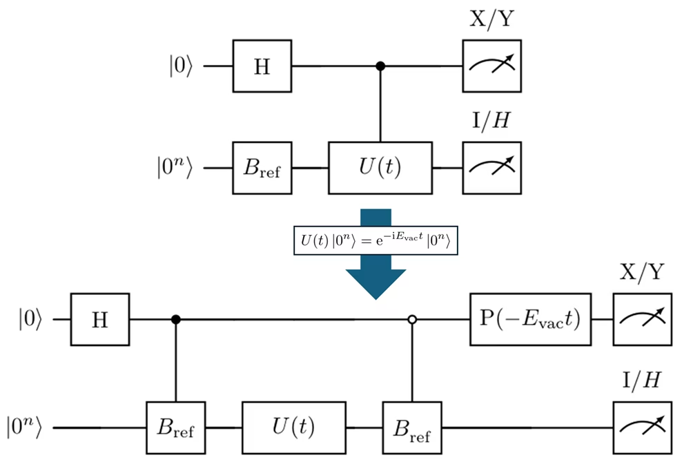
Qui, $B_{\rm ref}$ prepara lo stato di riferimento, $B_{\rm ref}|0^n\rangle = |\psi_{0}\rangle$.

Invece di preparare prima $\frac{1}{\sqrt{2}}(|0\rangle+|1\rangle)|\psi_0\rangle$ e poi applicare $U(t)$ solo sul ramo $|1\rangle$, il circuito prepara direttamente i due rami come

$$\begin{equation*} |0\rangle|\psi_0\rangle \quad \text{and} \quad |1\rangle|\psi_d\rangle , \end{equation*}$$

where

$$\begin{equation*} |\psi_d\rangle = U(d\Delta t)|\psi_0\rangle . \end{equation*}$$

Il circuito applica prima una porta di Hadamard all'ancilla e prepara lo stato di riferimento solo sul ramo $|1\rangle$:

$$\begin{equation*} |0\rangle |0^n\rangle \longrightarrow \frac{|0\rangle |0^n\rangle + |1\rangle B_{\rm ref}|0^n\rangle}{\sqrt{2}} = \frac{|0\rangle |0^n\rangle + |1\rangle |\psi_0\rangle}{\sqrt{2}} . \end{equation*}$$

Quindi l'operatore di evoluzione temporale non controllato viene applicato a entrambi i rami:

$$\begin{equation*} \frac{|0\rangle |0^n\rangle + |1\rangle |\psi_0\rangle}{\sqrt{2}} \longrightarrow \frac{|0\rangle U(t)|0^n\rangle + |1\rangle U(t)|\psi_0\rangle}{\sqrt{2}} . \end{equation*}$$

Poiché l'Hamiltoniana conserva il numero di eccitazioni, possiamo vedere che $|0^n\rangle$ è il suo autostato, e quindi l'operatore di evoluzione accumula solo una fase sotto l'Hamiltoniana:

$$\begin{equation*} U(t)|0^n\rangle = e^{-iE_{\rm vac}t}|0^n\rangle . \end{equation*}$$

Therefore,

$$\begin{equation*} \frac{|0\rangle U(t)|0^n\rangle + |1\rangle U(t)|\psi_0\rangle}{\sqrt{2}} = \frac{e^{-iE_{\rm vac}t}|0\rangle |0^n\rangle + |1\rangle U(t)|\psi_0\rangle}{\sqrt{2}} . \end{equation*}$$

Successivamente, $B_{\rm ref}$ viene applicato solo sul ramo $|0\rangle$.

$$\begin{equation*} \frac{e^{-iE_{\rm vac}t}|0\rangle |\psi_0\rangle + |1\rangle U(t)|\psi_0\rangle}{\sqrt{2}} . \end{equation*}$$

A questo punto, i due rami hanno una fase relativa aggiuntiva. Per rimuoverla, applichiamo la porta di fase dell'ancilla

$$\begin{equation*} P(-E_{\rm vac}t) = \begin{pmatrix} 1 & 0 \\ 0 & e^{-iE_{\rm vac}t} \end{pmatrix}. \end{equation*}$$

Questo trasforma lo stato come

$$\begin{equation*} \frac{e^{-iE_{\rm vac}t}|0\rangle |\psi_0\rangle + |1\rangle U(t)|\psi_0\rangle}{\sqrt{2}} \longrightarrow \frac{e^{-iE_{\rm vac}t}|0\rangle |\psi_0\rangle + e^{-iE_{\rm vac}t}|1\rangle U(t)|\psi_0\rangle}{\sqrt{2}} . \end{equation*}$$

Quindi, a meno di una fase globale irrilevante, abbiamo finalmente preparato

$$\begin{equation*} |\Phi_{0d}\rangle = \frac{ |0\rangle|\psi_0\rangle + |1\rangle U(t)|\psi_0\rangle }{\sqrt{2}} . \end{equation*}$$

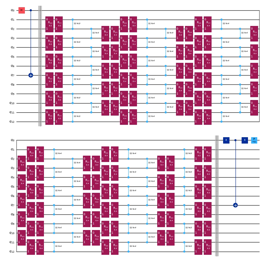
Nel prossimo blocco di codice, implementiamo questo circuito senza controllo.

controlled_extended_swap_test = extended_swap_test

# Reuse the ordering and synthesis rule selected by the comparison above.
evol_gate_optimized = PauliEvolutionGate(
    hamiltonian_for_synthesis,
    time=t,
    synthesis=SuzukiTrotter(order=2, reps=num_trotter_steps),
)

uncontrolled_evolution = QuantumCircuit(num_qubits, name="U_ST2(t)")
uncontrolled_evolution.append(evol_gate_optimized, range(num_qubits))

controlled_state_prep = QuantumCircuit(num_qubits + 1, name="C-Prep")
for q, bit in enumerate(reversed(ref_bitstring)):
    if bit == "1":
        controlled_state_prep.cx(ancilla, system_qubits[q])

vacuum_bitstring = "0" * num_qubits
vacuum_energy = basis_state_expectation_sparse(hamiltonian, "0" * num_qubits)

optimized_extended_swap_test = QuantumCircuit(num_qubits + 1)
optimized_extended_swap_test.h(ancilla)

# Prepare |psi_ref> only on the |1> branch.
optimized_extended_swap_test.compose(controlled_state_prep, inplace=True)
optimized_extended_swap_test.barrier()

# Apply the Trotterized time evolution without control.
optimized_extended_swap_test.compose(
    uncontrolled_evolution,
    qubits=system_qubits,
    inplace=True,
)
optimized_extended_swap_test.barrier()

# Map |0>|0...0> to |0>|psi_ref>, leaving the |1> branch unchanged.
optimized_extended_swap_test.x(ancilla)
optimized_extended_swap_test.compose(controlled_state_prep, inplace=True)
optimized_extended_swap_test.x(ancilla)

# Cancel the known vacuum phase so that the same X/Y observables can be used.
optimized_extended_swap_test.p(-vacuum_energy * t, ancilla)
optimized_extended_swap_test = simple_transpilation(
    optimized_extended_swap_test
)

print(f"Vacuum energy E_vac = {vacuum_energy:.1f}")
display(
    optimized_extended_swap_test.assign_parameters({t: 1.0}).draw(
        "mpl", scale=0.5, fold=26
    )
)

Vacuum energy E_vac = 11.0+0.0j

Transpilazione

Ora, transpiliamo i circuiti controllati e senza controllo per renderli eseguibili sull'hardware. Confrontiamo il risultato dei circuiti transpilati.

pass_manager = generate_preset_pass_manager(
    backend=backend,
    optimization_level=3,
)

isa_controlled_extended_swap_test = pass_manager.run(
    controlled_extended_swap_test
)

pass_manager = generate_preset_pass_manager(
    backend=backend, optimization_level=3, routing_method="none"
)
isa_optimized_extended_swap_test = pass_manager.run(
    optimized_extended_swap_test
)

transpilation_result = [
    {
        "label": "abstract controlled U(t)",
        **summarize_circuit(isa_controlled_extended_swap_test),
    },
    {
        "label": "optimized non-controlled U(t)",
        **summarize_circuit(isa_optimized_extended_swap_test),
    },
]

display(pd.DataFrame(transpilation_result))

def filter_qubits_from_layout(layout):
    q_layout = Layout(
        {
            physical: virtual
            for physical, virtual in layout.get_physical_bits().items()
            if virtual._register.name == "q"
        }
    )
    return q_layout

print(
    filter_qubits_from_layout(
        isa_optimized_extended_swap_test.layout.initial_layout
    )
)

isa_observables = [
    op.apply_layout(isa_optimized_extended_swap_test.layout)
    for op in observables
]

label  depth   size  2q gates  2q depth
0       abstract controlled U(t)  15457  23786      4686      4580
1  optimized non-controlled U(t)    261   1716       307        57

Layout({
18: <Qubit register=(13, "q"), index=0>,
5: <Qubit register=(13, "q"), index=1>,
6: <Qubit register=(13, "q"), index=2>,
7: <Qubit register=(13, "q"), index=3>,
8: <Qubit register=(13, "q"), index=4>,
9: <Qubit register=(13, "q"), index=5>,
10: <Qubit register=(13, "q"), index=6>,
11: <Qubit register=(13, "q"), index=7>,
12: <Qubit register=(13, "q"), index=8>,
13: <Qubit register=(13, "q"), index=9>,
14: <Qubit register=(13, "q"), index=10>,
15: <Qubit register=(13, "q"), index=11>,
19: <Qubit register=(13, "q"), index=12>
})

Step 3: Eseguire utilizzando le primitive di Qiskit

Il passo successivo è sottoporre lo stesso circuito parametrizzato per diversi valori di $d$. Per ciascun $d$, stimiamo quattro valori di aspettazione: $X\otimes I$, $Y\otimes I$, $X\otimes (H-T)$ e $Y\otimes (H-T)$. Questi quattro numeri vengono poi combinati negli elementi complessi della prima riga $\mathcal{S}_{0d}$ e $\mathcal{H}_{0d}$.

Qui, $\mathcal{S}_{00}=1$ e $\mathcal{H}_{00}=\langle\psi_{0}|(H-T)|\psi_{0}\rangle=\langle\psi_{0}|H|\psi_{0}\rangle-\tau$ possono essere calcolati classicamente poiché $\lvert\psi_0\rangle$ è sparso, quindi saltiamo il caso $d=0$.

pub_list = []
d_values = list(range(1, krylov_dim))

# Exact local statevector estimator.
estimator = StatevectorEstimator()

# We use the circuit before the transpilation for the local simulator,
# but we will use the transpiled circuit for the real backend.
for d in d_values:
    parameter_values = [d * dt]

    for ob in observables:
        pub_list.append(
            (
                optimized_extended_swap_test,
                ob,
                parameter_values,
            )
        )

job = estimator.run(pub_list)

# Local PrimitiveJob does not provide Runtime-style job inputs,
# so preserve the inputs directly.
inputs = pub_list
result = job.result()

print(f"Number of Krylov basis states: r = {len(d_values)}")
print(f"Number of PUBs: {len(pub_list)}")
print(f"Each d uses observables: {observable_labels}")

Number of Krylov basis states: r = 9
Number of PUBs: 36
Each d uses observables: ['Re S_0d', 'Im S_0d', 'Re shifted H_0d', 'Im shifted H_0d']

Step 4: Post-elaborazione e restituzione del risultato in formato classico desiderato

Dopo aver stimato le matrici proiettate, regolarizziamo e risolviamo il GEVP

$$\begin{equation*} \mathcal{H}\mathbf{c} = E\mathcal{S}\mathbf{c}. \end{equation*}$$

Il più piccolo autovalore generalizzato fornisce la stima KQD dell'energia dello stato fondamentale.

h_shifted_row_est = np.zeros(krylov_dim, dtype=complex)
s_row_est = np.zeros(krylov_dim, dtype=complex)

h_shifted_row_est[0] = ref_energy - shift_tau
s_row_est[0] = 1.0

for idx, (pub_input, pub_result) in enumerate(zip(inputs, result)):
    d_index, obs_index = divmod(idx, len(observables))
    ev = np.asarray(pub_result.data.evs).reshape(-1)[0]
    std = np.asarray(pub_result.data.stds).reshape(-1)[0]

    if obs_index == 0:
        s_row_est[d_index + 1] = ev
    elif obs_index == 1:
        s_row_est[d_index + 1] += 1j * ev
    elif obs_index == 2:
        h_shifted_row_est[d_index + 1] = ev
    elif obs_index == 3:
        h_shifted_row_est[d_index + 1] += 1j * ev

# H_0d = shifted_H_0d + tau * S_0d.
h_row_est = h_shifted_row_est + shift_tau * s_row_est

h_matrix_est = la.toeplitz(h_row_est.conj(), h_row_est)
s_matrix_est = la.toeplitz(s_row_est.conj(), s_row_est)

s_eigvals = la.eigvalsh(0.5 * (s_matrix_est + s_matrix_est.conj().T))
positive_s_eigvals = s_eigvals[s_eigvals > 1e-12]
s_condition_number = (
    positive_s_eigvals[-1] / positive_s_eigvals[0]
    if len(positive_s_eigvals) > 0
    else np.inf
)

with np.printoptions(precision=3, suppress=True):
    print("Estimated first row of S:")
    print(s_row_est)
    print()
    print("Estimated first row of H:")
    print(h_row_est)
    print()
    print("Eigenvalues of the estimated overlap matrix S:")
    print(s_eigvals)
    print(f"Condition number above 1e-12: {s_condition_number:.3e}")
    print()

Estimated first row of S:
[ 1.   +0.j     0.758-0.596j  0.203-0.836j -0.291-0.636j -0.444-0.229j
 -0.276+0.053j -0.044+0.051j  0.006-0.121j -0.155-0.218j -0.345-0.101j]

Estimated first row of H:
[ 7.   +0.j     4.842-4.76j   0.044-6.185j -3.791-3.653j -4.137+0.39j
 -1.495+2.654j  1.331+1.777j  1.85 -0.763j -0.032-2.278j -2.222-1.372j]

Eigenvalues of the estimated overlap matrix S:
[-0.     0.     0.     0.     0.     0.     0.01   0.355  3.526  6.109]
Condition number above 1e-12: 1.904e+12

Ora risolviamo il problema agli autovalori generalizzato utilizzando le matrici ricostruite dalle stime del circuito. In un calcolo ideale di statevector con evoluzione esatta in tempo reale, questo dovrebbe riprodurre il risultato proiettato esatto. In pratica, le deviazioni possono derivare dalla Trotterizzazione, dall'errore di campionamento e dall'instabilità numerica della matrice di overlap.

Osserviamo come l'energia converge man mano che aumentiamo la dimensione del sottospazio di Krylov.

exact_evals = diagonalize_single_1_subspace(hamiltonian)
exact_ground = min(exact_evals)
print("exact ground state energy:  ", exact_ground)

threshold = 1e-12
energy_convergence = []

for r in range(1, krylov_dim + 1):
    energy_est_kqd, coeffs_est, retained_est = solve_thresholded_gevp(
        h_matrix_est[:r, :r],
        s_matrix_est[:r, :r],
        threshold=threshold,
    )
    energy_convergence.append(energy_est_kqd)
    print(
        f"Krylov ground state energy (dim={r}, retained={retained_est}): ",
        energy_est_kqd,
    )

exact ground state energy:   3.136296694843727
Krylov ground state energy (dim=1, retained=1):  7.0
Krylov ground state energy (dim=2, retained=2):  4.184510657551266
Krylov ground state energy (dim=3, retained=3):  3.5539074630394136
Krylov ground state energy (dim=4, retained=4):  3.3366270761341044
Krylov ground state energy (dim=5, retained=5):  3.252017453225087
Krylov ground state energy (dim=6, retained=6):  3.2300275138879186
Krylov ground state energy (dim=7, retained=7):  3.2299154099085685
Krylov ground state energy (dim=8, retained=7):  3.2298063744216776
Krylov ground state energy (dim=9, retained=7):  3.2296778282872456
Krylov ground state energy (dim=10, retained=8):  3.223647515867734

def plot_energy_convergence(energy_convergence, exact_ground, krylov_dim):
    fig, ax = plt.subplots(figsize=(7, 4.5))

    ax.plot(
        range(1, krylov_dim + 1),
        energy_convergence,
        marker="o",
        label="KQD estimate",
    )

    ax.axhline(
        exact_ground,
        linestyle="--",
        label=f"Exact ground energy = {exact_ground:.6f}",
    )

    ax.set_xlabel("Krylov dimension")
    ax.set_ylabel("Ground-state energy")
    ax.grid(True, alpha=0.3)
    ax.legend()
    plt.tight_layout()
    plt.show()

plot_energy_convergence(energy_convergence, exact_ground, krylov_dim)

Esempio hardware su larga scala

La sezione precedente ha utilizzato un modello a 12 qubit in modo che la simulazione statevector potesse essere utilizzata come diagnostica. Ora scaliamo lo stesso workflow KQD a una catena di Heisenberg a 30 qubit e prepariamo il carico di lavoro per l'esecuzione su hardware IBM Quantum.

Step 1-4 compressi in un singolo blocco di codice

Qui mettiamo insieme tutti questi dettagli in un unico workflow su scala più grande, che viene poi eseguito sul nostro hardware quantistico reale. In questa sezione, applichiamo impostazioni realistiche di mitigazione degli errori per migliorare l'affidabilità dei risultati. Poiché gli elementi di matrice corrispondenti a diversi valori di $d$ possono essere valutati in parallelo, utilizziamo la modalità Batch per eseguirli in modo efficiente.

# -------------------------Step 1-------------------------

# Map the classical problem to quantum circuits and observables.
# Problem and KQD parameters.
large_num_qubits = 30
large_krylov_dim = 7
large_num_trotter_steps = 3
large_dt = np.pi / (3 * (large_num_qubits - 1))
large_t = Parameter("t_large")

# Use a single excitation near the center of the chain.
large_excitation_qubit = large_num_qubits // 2
large_ref_label = ["0"] * large_num_qubits
large_ref_label[large_num_qubits - 1 - large_excitation_qubit] = "1"
large_ref_bitstring = "".join(large_ref_label)

# Use the ordering and product formula selected in the preceding section.
large_hamiltonian = make_heisenberg_hamiltonian_ordered(
    large_num_qubits,
    ordering="even-odd edge-grouped",
    coupling=1.0,
)
large_ref_energy = float(
    np.real(
        basis_state_expectation_sparse(large_hamiltonian, large_ref_bitstring)
    )
)
large_vacuum_energy = float(
    np.real(
        basis_state_expectation_sparse(
            large_hamiltonian, "0" * large_num_qubits
        )
    )
)

large_evolution_gate = PauliEvolutionGate(
    large_hamiltonian,
    time=large_t,
    synthesis=SuzukiTrotter(order=2, reps=large_num_trotter_steps),
)
large_uncontrolled_evolution = QuantumCircuit(
    large_num_qubits,
    name="U_ST2_large(t)",
)
large_uncontrolled_evolution.append(
    large_evolution_gate,
    range(large_num_qubits),
)

# Build the control-free extended-swap-test circuit.
large_ancilla = 0
large_system_qubits = list(range(1, large_num_qubits + 1))

large_controlled_state_prep = QuantumCircuit(
    large_num_qubits + 1,
    name="C-Prep-large",
)
large_controlled_state_prep.cx(
    large_ancilla,
    large_system_qubits[large_excitation_qubit],
)

large_extended_swap_test = QuantumCircuit(large_num_qubits + 1)
large_extended_swap_test.h(large_ancilla)
large_extended_swap_test.compose(large_controlled_state_prep, inplace=True)
large_extended_swap_test.compose(
    large_uncontrolled_evolution,
    qubits=large_system_qubits,
    inplace=True,
)
large_extended_swap_test.x(large_ancilla)
large_extended_swap_test.compose(
    large_controlled_state_prep.inverse(),
    inplace=True,
)
large_extended_swap_test.x(large_ancilla)
large_extended_swap_test.p(
    -large_vacuum_energy * large_t,
    large_ancilla,
)

# Reuse the Hamiltonian-shifting construction from the preceding section.
(
    large_obs_x_shifted_hamiltonian,
    large_obs_y_shifted_hamiltonian,
    large_shift_tau,
) = make_reduced_heisenberg_observables(large_ref_bitstring)

large_observables = [
    SparsePauliOp("I" * large_num_qubits + "X"),
    SparsePauliOp("I" * large_num_qubits + "Y"),
    large_obs_x_shifted_hamiltonian,
    large_obs_y_shifted_hamiltonian,
]
large_observable_labels = [
    "Re S_0d",
    "Im S_0d",
    "Re shifted H_0d",
    "Im shifted H_0d",
]

# -------------------------Step 2-------------------------

# Optimize the problem for quantum execution.
# Select a real backend and transpile the parameterized circuit to ISA form.
large_backend = service.backend("ibm_boston")
large_pass_manager = generate_preset_pass_manager(
    backend=large_backend, optimization_level=3, routing_method="none"
)
large_isa_circuit = large_pass_manager.run(large_extended_swap_test)
large_isa_observables = [
    observable.apply_layout(large_isa_circuit.layout)
    for observable in large_observables
]

large_two_qubit_gate_count = sum(
    instruction.operation.num_qubits == 2
    for instruction in large_isa_circuit.data
)

print(f"Backend: {large_backend.name}")
print(f"System qubits: {large_num_qubits}")
print(f"Total circuit qubits: {large_isa_circuit.num_qubits}")
print(f"Krylov dimension: {large_krylov_dim}")
print(f"Time step: {large_dt:.6f}")
print(f"Shift tau: {large_shift_tau}")
print(f"ISA circuit depth: {large_isa_circuit.depth()}")
print(f"ISA two-qubit gates: {large_two_qubit_gate_count}")
print(
    f"ISA two-qubit depth: {large_isa_circuit.depth(lambda x: x[0].num_qubits == 2)}"
)

# -------------------------Step 3-------------------------

# Execute on quantum hardware with Qiskit Runtime primitives.
# Submit one job per d, with all four observables in that job.
large_d_values = list(range(1, large_krylov_dim))
retrieve_batch_id = None
large_jobs = []

if retrieve_batch_id is None:
    large_estimator_options = {
        "default_shots": 8192,
        "dynamical_decoupling": {
            "enable": True,
            "sequence_type": "XpXm",
        },
        "resilience": {
            "measure_mitigation": True,
            "measure_noise_learning": {
                "num_randomizations": 32,
                "shots_per_randomization": 256,
            },
            "layer_noise_learning": {
                "max_layers_to_learn": 4,
                "layer_pair_depths": [0, 1, 2, 4, 16, 32],
                "num_randomizations": 32,
                "shots_per_randomization": 128,
            },
            "zne_mitigation": True,
            "zne": {
                "amplifier": "pea",
                "noise_factors": [1.0, 1.5, 2.0],
                "extrapolator": ("exponential", "linear"),
            },
        },
        "twirling": {
            "enable_gates": True,
            "enable_measure": True,
            "num_randomizations": 32,
            "shots_per_randomization": 256,
            "strategy": "active-accum",
        },
    }

    with Batch(backend=large_backend) as large_batch:
        large_batch_id = large_batch.session_id
        large_estimator = EstimatorV2(
            mode=large_batch,
            options=large_estimator_options,
        )
        # Krylov quantum diagonalization of lattice Hamiltonians -> TUT_KQDOLH.
        large_estimator.options.environment.job_tags = ["TUT_KQDOLH"]

        for d in large_d_values:
            parameter_values = [d * large_dt]
            pubs_for_d = [
                (large_isa_circuit, observable, parameter_values)
                for observable in large_isa_observables
            ]
            job = large_estimator.run(pubs_for_d)
            large_jobs.append(job)
            print(
                f"Submitted d={d}: job_id={job.job_id()}, "
                f"PUBs={len(pubs_for_d)}"
            )

    print(f"Batch ID: {large_batch_id}")
else:
    large_batch_id = retrieve_batch_id
    large_jobs = service.jobs(
        session_id=large_batch_id,
        limit=None,
        descending=False,
    )

large_job_ids_by_d = {
    d: job.job_id() for d, job in zip(large_d_values, large_jobs)
}
print(f"Job IDs by d: {large_job_ids_by_d}")

# -------------------------Step 4-------------------------

# Post-process the quantum results and solve the classical GEVP.
# Reconstruct the first rows of S and the shifted Hamiltonian matrix.
large_s_row_est = np.zeros(large_krylov_dim, dtype=complex)
large_h_shifted_row_est = np.zeros(large_krylov_dim, dtype=complex)
large_s_row_est[0] = 1.0
large_h_shifted_row_est[0] = large_ref_energy - large_shift_tau

for d, job in zip(large_d_values, large_jobs):
    job_result = job.result()

    if len(job_result) != len(large_observables):
        raise RuntimeError(
            f"Expected {len(large_observables)} PUB results for d={d}, "
            f"but received {len(job_result)}."
        )

    expectation_values = [
        np.asarray(pub_result.data.evs).reshape(-1)[0]
        for pub_result in job_result
    ]

    large_s_row_est[d] = expectation_values[0] + 1j * expectation_values[1]
    large_h_shifted_row_est[d] = (
        expectation_values[2] + 1j * expectation_values[3]
    )

# H_0d = shifted_H_0d + tau * S_0d.
large_h_row_est = large_h_shifted_row_est + large_shift_tau * large_s_row_est

large_s_matrix_est = la.toeplitz(
    large_s_row_est.conj(),
    large_s_row_est,
)
large_h_matrix_est = la.toeplitz(
    large_h_row_est.conj(),
    large_h_row_est,
)

large_exact_gnd = min(diagonalize_single_1_subspace(large_hamiltonian))

large_energy_convergence = []

with np.printoptions(precision=5, suppress=True):
    print("Estimated first row of S:")
    print(large_s_row_est)
    print("Estimated first row of H:")
    print(large_h_row_est)
    print("exact ground state energy:  ", large_exact_gnd)

    for r in range(1, large_krylov_dim + 1):
        energy_est_kqd, coeffs_est, retained_est = solve_thresholded_gevp(
            large_h_matrix_est[:r, :r],
            large_s_matrix_est[:r, :r],
            threshold=5e-2,
        )
        large_energy_convergence.append(energy_est_kqd)
        print(
            f"Krylov ground state energy (dim={r}, retained={retained_est}): ",
            energy_est_kqd,
        )

plot_energy_convergence(
    large_energy_convergence, large_exact_gnd, large_krylov_dim
)

Backend: ibm_boston
System qubits: 30
Total circuit qubits: 156
Krylov dimension: 7
Time step: 0.036110
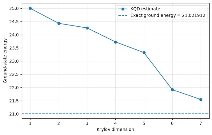
Shift tau: 25.0
ISA circuit depth: 219
ISA two-qubit gates: 728
ISA two-qubit depth: 52
Job IDs by d: {1: 'd9fl4p4jeosc73fk4dg0', 2: 'd9fl4pineu4c739poecg', 3: 'd9fl4q2neu4c739poedg', 4: 'd9fl4qhhtsac739fjgn0', 5: 'd9fl4r4jeosc73fk4dhg', 6: 'd9fl4rkjeosc73fk4dj0'}
Estimated first row of S:
[ 1.     +0.j       0.42055-0.65466j -0.17883-0.73125j -0.64523-0.31601j
 -0.70781+0.55574j -0.02467+0.70525j  0.59301+0.55602j]
Estimated first row of H:
[ 25.      +0.j       10.3419 -16.5586j   -5.017  -18.03933j
 -16.44797 -6.98173j -17.17081+14.84502j   0.62722+17.81196j
  15.68886+12.74875j]
exact ground state energy:   21.021912418526902
Krylov ground state energy (dim=1, retained=1):  25.0
Krylov ground state energy (dim=2, retained=2):  24.432409110686205
Krylov ground state energy (dim=3, retained=3):  24.256856893278556
Krylov ground state energy (dim=4, retained=4):  23.727409826799715
Krylov ground state energy (dim=5, retained=4):  23.324720470780864
Krylov ground state energy (dim=6, retained=5):  21.91957579005085
Krylov ground state energy (dim=7, retained=5):  21.548331214122644

Appendice: Il punto di vista della funzione Hamiltoniana (filtro spettrale)

Il workflow principale ha presentato la KQD in modo operativo: costruire una base di Krylov da stati evoluti in tempo reale, stimare le matrici proiettate $\mathcal{H}$ e $\mathcal{S}$, e risolvere il GEVP. Questa appendice rivisita lo stesso calcolo da un'angolazione complementare che spiega perché la KQD funziona: il punto di vista della funzione Hamiltoniana, ovvero il filtro spettrale [3], [5]. Riutilizza il modello a 12 qubit, il passo temporale $\Delta t$, e la soluzione di Krylov già ottenuta sopra; non è richiesta alcuna nuova esecuzione di circuiti.

Lo stato di riferimento come distribuzione di energia

Sia l'Hamiltoniana con la decomposizione agli autovalori

$$\begin{equation*} H=\sum_{m} E_m\,|E_m\rangle\!\langle E_m|, \qquad E_0\le E_1\le\cdots, \end{equation*}$$

con autostati energetici $|E_m\rangle$. Ogni stato di riferimento può essere espanso in questa autobase,

$$\begin{equation*} |\psi_{0}\rangle=\sum_m a_m\,|E_m\rangle, \qquad a_m=\langle E_m|\psi_{0}\rangle, \end{equation*}$$

quindi porta un peso spettrale $p_m=|a_m|^2$ a ciascuna energia $E_m$. L'energia di riferimento è la media di questa distribuzione, $\langle H\rangle_{0}=\sum_m p_m E_m$.

L'autodecomposizione di un'Hamiltoniana generale a $n$ qubit ha un costo esponenziale, quindi questa rappresentazione è solo diagnostica, e non fa parte dell'algoritmo. Qui, tuttavia, possiamo calcolarla in modo economico per lo stesso problema con $n=12$: l'Hamiltoniana di Heisenberg conserva il numero totale di eccitazioni, e il riferimento $|000001000000\rangle$ porta una singola eccitazione, quindi tutto il suo contenuto spettrale vive nel sottospazio a singola eccitazione, la cui dimensione cresce solo linearmente con $n$. Riutilizziamo quindi il blocco esatto a singola eccitazione (già usato sopra come benchmark) e leggiamo la distribuzione di riferimento $\{(E_m, p_m)\}$ all'interno di quel sottospazio.

# Exact single-excitation-subspace decomposition of the reference state.
# This reuses make_heisenberg_hamiltonian / _basis_state_transition_amplitude_sparse
# and the n=12 `hamiltonian` and `ref_bitstring` defined in the small-scale example.
single_excitation_states = [1 << k for k in range(num_qubits)]

h_single = np.array(
    [
        [
            _basis_state_transition_amplitude_sparse(hamiltonian, bra, ket)
            for ket in single_excitation_states
        ]
        for bra in single_excitation_states
    ]
)
h_single = 0.5 * (h_single + h_single.conj().T)

subspace_evals, subspace_evecs = la.eigh(h_single)
subspace_evals = np.real(subspace_evals)

# Reference-state coordinates inside the single-excitation subspace.
ref_position = single_excitation_states.index(int(ref_bitstring, 2))
ref_in_subspace = np.zeros(num_qubits, dtype=complex)
ref_in_subspace[ref_position] = 1.0

# Amplitudes and spectral weights of the reference in the energy eigenbasis.
ref_eigen_amplitudes = subspace_evecs.conj().T @ ref_in_subspace
ref_spectral_weights = np.abs(ref_eigen_amplitudes) ** 2

print(f"Single-excitation subspace dimension: {num_qubits}")
print(f"Subspace ground-state energy:         {subspace_evals[0]:.6f}")
print(
    f"Reference energy (sum p_m E_m):       {np.sum(ref_spectral_weights * subspace_evals):.6f}"
)
print(f"Reference weight on subspace ground:  {ref_spectral_weights[0]:.6f}")

Single-excitation subspace dimension: 12
Subspace ground-state energy:         3.136297
Reference energy (sum p_m E_m):       7.000000
Reference weight on subspace ground:  0.163827

KQD apprende un filtro che rimodella questa distribuzione

Una funzione Hamiltoniana $f(H)$ è definita tramite il calcolo spettrale,

$$\begin{equation*} f(H)=\sum_m f(E_m)\,|E_m\rangle\!\langle E_m|, \end{equation*}$$

ovvero, in altre parole, una somma pesata di autoproiettori. Applicarla al riferimento rimodella ciascuna ampiezza spettrale, $a_m \to a_m f(E_m)$:

$$\begin{equation*} f(H)\,|\psi_{0}\rangle=\sum_m a_m\,f(E_m)\,|E_m\rangle . \end{equation*}$$

Se $f$ fosse fortemente concentrata all'energia più bassa ($f(E_0)=1$ e $f(E_m)\approx 0$ altrimenti), allora $f(H)$ agirebbe come un proiettore sullo stato fondamentale, e l'output normalizzato sarebbe (vicino a) lo stato fondamentale. Pertanto, un buon filtro spettrale passa-basso in energia è esattamente ciò che vogliamo.

KQD non prescrive $f$ in anticipo. Invece espande il filtro nella base dell'evoluzione temporale reale,

$$\begin{equation*} f_{\rm KQD}(E)=\sum_{\ell=0}^{r-1} c_\ell\, e^{-i\ell\Delta t E}, \end{equation*}$$

una funzione trigonometrica dell'energia i cui coefficienti $\{c_\ell\}$ sono precisamente l'autovettore del GEVP risolto sopra. Minimizzare il quoziente di Rayleigh $\mathbf{c}^\dagger\mathcal{H}\mathbf{c}/\mathbf{c}^\dagger\mathcal{S}\mathbf{c}$ equivale quindi a imparare il filtro che meglio sopprime il peso degli stati eccitati del riferimento. Una dimensione di Krylov $r$ maggiore dà al filtro più gradi di libertà e un picco più netto all'energia dello stato fondamentale.

L'helper qui sotto valuta questo filtro appreso su un asse energetico; lo applichiamo poi alla distribuzione di riferimento ottenuta sopra.

def trigonometric_krylov_filter(
    coeffs: np.ndarray,
    energies: np.ndarray,
    time_step: float,
) -> np.ndarray:
    """Evaluate the learned Krylov filter f(E) = sum_l c_l exp(-i l dt E)."""
    values = np.zeros_like(energies, dtype=complex)
    for ell, coeff in enumerate(coeffs):
        values += coeff * np.exp(-1j * ell * time_step * energies)
    return values

def filtered_spectral_weights(
    weights: np.ndarray,
    filter_values: np.ndarray,
) -> np.ndarray:
    """Reshape spectral weights by |f(E)|^2 and renormalize."""
    reshaped = weights * np.abs(filter_values) ** 2
    return reshaped / np.sum(reshaped)

# Recover the KQD coefficients from the already-estimated projected matrices.
# The shift only moves H by tau * S, so it does not change the GEVP eigenvector;
# we solve at the full Krylov dimension used in the small-scale example.
_, kqd_coeffs, _ = solve_thresholded_gevp(
    h_matrix_est,
    s_matrix_est,
    threshold=1e-12,
)

filter_on_spectrum = trigonometric_krylov_filter(
    kqd_coeffs, subspace_evals, dt
)
filtered_weights = filtered_spectral_weights(
    ref_spectral_weights, filter_on_spectrum
)

print(f"Ground-state overlap  (reference): {ref_spectral_weights[0]:.4f}")
print(f"Ground-state overlap  (filtered):  {filtered_weights[0]:.4f}")
print(
    f"Mean energy           (reference): {np.sum(ref_spectral_weights * subspace_evals):.6f}"
)
print(
    f"Mean energy           (filtered):  {np.sum(filtered_weights * subspace_evals):.6f}"
)

Ground-state overlap  (reference): 0.1638
Ground-state overlap  (filtered):  0.9638
Mean energy           (reference): 7.000000
Mean energy           (filtered):  3.164503

Visualizza il filtro e la sua flessibilità

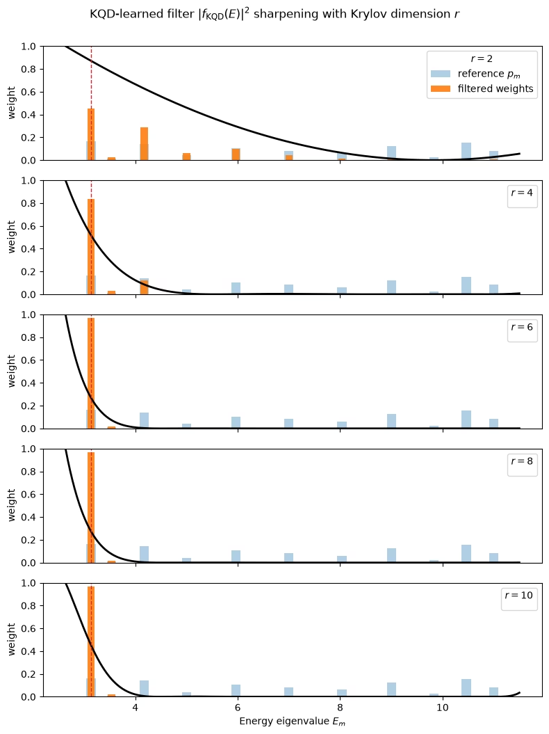
Mostriamo prima il filtro appreso alla dimensione di Krylov piena usata sopra, poi osserviamo come si affina al crescere della dimensione $r$.

Le barre mostrano i pesi spettrali di riferimento $p_m$ (prima) e i pesi filtrati $p_m|f_{\rm KQD}(E_m)|^2$ (dopo), insieme all'intensità del filtro appreso $|f_{\rm KQD}(E)|^2$ su un asse energetico continuo. Il filtro concentra il peso sull'energia più bassa del sottospazio a singola eccitazione — la stessa energia a cui è conversa la stima KQD nell'esempio su piccola scala. Nota che questo è lo stato fondamentale all'interno del settore a singola eccitazione, che è l'obiettivo rilevante per questo stato di riferimento che conserva le eccitazioni, non lo stato fondamentale globale.

fig, ax = plt.subplots(figsize=(8, 4))

visible = (ref_spectral_weights > 1e-4) | (filtered_weights > 1e-4)
ax.bar(
    subspace_evals[visible],
    ref_spectral_weights[visible],
    width=0.18,
    alpha=0.45,
    label="reference $p_m$",
)
ax.bar(
    subspace_evals[visible],
    filtered_weights[visible],
    width=0.14,
    alpha=0.9,
    label=r"filtered $p_m\,|f_{\rm KQD}(E_m)|^2$",
)

energy_grid = np.linspace(
    subspace_evals.min() - 0.5, subspace_evals.max() + 0.5, 800
)
filter_intensity = (
    np.abs(trigonometric_krylov_filter(kqd_coeffs, energy_grid, dt)) ** 2
)
filter_intensity /= filter_intensity.max()
ax.plot(
    energy_grid,
    filter_intensity,
    color="k",
    linewidth=2,
    label=r"$|f_{\rm KQD}(E)|^2$ (normalized)",
)

ax.axvline(
    subspace_evals[0],
    color="C3",
    linestyle="--",
    linewidth=1,
    label="subspace ground energy",
)
ax.set_xlabel("Energy eigenvalue $E_m$")
ax.set_ylabel("Spectral weight")
ax.set_ylim(0, 1)
ax.legend(loc="upper right")
plt.tight_layout()
plt.show()

Aumentare la dimensione di Krylov: flessibilità della funzione appresa

Ricorda che il filtro appreso è un polinomio trigonometrico nell'energia con $r$ coefficienti,

$$\begin{equation*} f_{\rm KQD}(E)=\sum_{\ell=0}^{r-1} c_\ell\, e^{-i\ell\Delta t E}. \end{equation*}$$

La dimensione di Krylov $r$ è esattamente il numero di coefficienti liberi, quindi controlla la flessibilità della funzione. Un $r$ piccolo può produrre solo un filtro ampio e variabile dolcemente, che lascia trapelare peso verso stati eccitati di bassa energia; quando $r$ aumenta, il filtro può formare un picco più stretto all'energia target e sopprimere in modo più aggressivo il peso residuo degli stati eccitati. Questa è la controparte, in termini di filtro spettrale, della convergenza in energia osservata nell'esempio su piccola scala: al crescere di $r$, la distribuzione filtrata collassa sullo stato fondamentale del sottospazio e l'energia stimata diminuisce verso di esso.

Riutilizziamo le matrici proiettate già stimate sopra e risolviamo semplicemente il GEVP su ciascun blocco principale $r\times r$, quindi valutiamo e tracciamo il filtro corrispondente.

# Sweep the Krylov dimension using the leading r x r blocks of the estimated matrices.
sweep_dims = [r for r in (2, 4, 6, 8, krylov_dim) if r <= krylov_dim]
sweep_dims = sorted(set(sweep_dims))

energy_grid = np.linspace(
    subspace_evals.min() - 0.5, subspace_evals.max() + 0.5, 800
)

sweep_cases = []
print(" r    retained    ground overlap    filtered energy")
print("--    --------    --------------    ---------------")
for r in sweep_dims:
    _, coeffs_r, retained_r = solve_thresholded_gevp(
        h_matrix_est[:r, :r],
        s_matrix_est[:r, :r],
        threshold=1e-12,
    )
    filter_on_spectrum_r = trigonometric_krylov_filter(
        coeffs_r, subspace_evals, dt
    )
    filtered_weights_r = filtered_spectral_weights(
        ref_spectral_weights, filter_on_spectrum_r
    )
    filtered_energy_r = float(np.sum(filtered_weights_r * subspace_evals))

    sweep_cases.append((r, coeffs_r, filtered_weights_r))
    print(
        f"{r:2d}    {retained_r:8d}    {filtered_weights_r[0]:14.4f}    {filtered_energy_r:15.6f}"
    )

print(f"\nSubspace ground-state energy (target): {subspace_evals[0]:.6f}")

# One panel per Krylov dimension: filtered spectrum (bars) + filter intensity (curve).
fig, axes = plt.subplots(
    len(sweep_cases),
    1,
    figsize=(8, 2.1 * len(sweep_cases)),
    sharex=True,
)
axes = np.atleast_1d(axes)

for idx, (ax, (r, coeffs_r, filtered_weights_r)) in enumerate(
    zip(axes, sweep_cases)
):
    visible = (ref_spectral_weights > 1e-4) | (filtered_weights_r > 1e-4)
    ax.bar(
        subspace_evals[visible],
        ref_spectral_weights[visible],
        width=0.18,
        alpha=0.35,
        color="C0",
        label="reference $p_m$" if idx == 0 else None,
    )
    ax.bar(
        subspace_evals[visible],
        filtered_weights_r[visible],
        width=0.14,
        alpha=0.9,
        color="C1",
        label="filtered weights" if idx == 0 else None,
    )

    filter_intensity_r = (
        np.abs(trigonometric_krylov_filter(coeffs_r, energy_grid, dt)) ** 2
    )
    filter_intensity_r /= filter_intensity_r.max()
    ax.plot(energy_grid, filter_intensity_r, color="k", linewidth=2)

    ax.axvline(subspace_evals[0], color="C3", linestyle="--", linewidth=1)
    ax.set_ylim(0, 1)
    ax.set_ylabel("weight")
    ax.legend(loc="upper right", title=f"$r={r}$")

axes[-1].set_xlabel("Energy eigenvalue $E_m$")
fig.suptitle(
    r"KQD-learned filter $|f_{\rm KQD}(E)|^2$ sharpening with Krylov dimension $r$",
    y=1.0,
)
fig.tight_layout()
plt.show()

r    retained    ground overlap    filtered energy
--    --------    --------------    ---------------
 2           2            0.4549           4.184510
 4           4            0.8373           3.310168
 6           6            0.9706           3.158100
 8           7            0.9701           3.158725
10           8            0.9638           3.164503

Subspace ground-state energy (target): 3.136297

Prossimi passi

Se hai trovato interessante questo lavoro, potresti essere interessato al seguente materiale:

Consigli

• Diagonalizzazione quantistica di Krylov basata su campionamento di un modello reticolare fermionico
• Stima dell'energia dello stato fondamentale della catena di Heisenberg con VQE
• Corso sugli algoritmi di diagonalizzazione quantistica

Riferimenti

[1] E. N. Epperly, L. Lin, and Y. Nakatsukasa, A theory of quantum subspace diagonalization, SIAM Journal on Matrix Analysis and Applications 43, 1263-1290 (2022).

[2] N. Yoshioka, M. Amico, W. Kirby, et al., Diagonalization of large many-body Hamiltonians on a quantum processor, arXiv:2407.14431 (2024).

[3] R. M. Parrish e P. L. McMahon, Quantum filter diagonalization: quantum eigendecomposition without full quantum phase estimation, Physical Review Letters 122, 230401 (2019).

[4] G. Lee, S. Choi, J. Huh, e A. F. Izmaylov, Efficient strategies for reducing sampling error in quantum Krylov subspace diagonalization, Digital Discovery 4, 954-969 (2025).

[5] G. Lee, M. Kang, J. Hong, S. Fomichev e J. Huh, Filtered Quantum Phase Estimation, arXiv:2510.04294 (2025).