Esperimento su scala utility III

nota

Toshinari Itoko, Tamiya Onodera, Kifumi Numata (19 luglio 2024)

Scarica il PDF della lezione originale. Nota che alcuni frammenti di codice potrebbero essere diventati obsoleti poiché si tratta di immagini statiche.

Il tempo QPU approssimativo per eseguire questo primo esperimento è di 12 min 30 s. C'è un esperimento aggiuntivo di seguito che richiede circa 4 min.

(Nota: questo notebook potrebbe non completare l'esecuzione nel tempo consentito dal Piano Open. Assicurati di usare le risorse di quantum computing in modo oculato.)

# Added by doQumentation — required packages for this notebook
!pip install -q numpy qiskit qiskit-ibm-runtime rustworkx

import qiskit

qiskit.__version__

'2.0.2'

import qiskit_ibm_runtime

qiskit_ibm_runtime.__version__

'0.40.1'

import numpy as np
import rustworkx as rx

from qiskit import QuantumCircuit
from qiskit.visualization import plot_histogram
from qiskit.visualization import plot_gate_map
from qiskit.transpiler.preset_passmanagers import generate_preset_pass_manager
from qiskit.providers import BackendV2
from qiskit.quantum_info import SparsePauliOp

from qiskit_ibm_runtime import QiskitRuntimeService
from qiskit_ibm_runtime import Sampler, Estimator, Batch, SamplerOptions

1. Introduzione

Facciamo un breve ripasso degli stati GHZ e di quale tipo di distribuzione ci si potrebbe aspettare dal Sampler applicato a uno di essi. Poi enunceremo esplicitamente l'obiettivo di questa lezione.

1.1 Stato GHZ

Lo stato GHZ (stato di Greenberger-Horne-Zeilinger) per $n$ qubit è definito come

$$\frac{1}{\sqrt 2}(|0\rangle ^ {\otimes n}+ |1\rangle^ {\otimes n})$$

Naturalmente, può essere creato per 6 qubit con il seguente circuito quantistico.

N = 6
qc = QuantumCircuit(N, N)

qc.h(0)
for i in range(N - 1):
    qc.cx(0, i + 1)

# qc.measure_all()
qc.barrier()
qc.measure(list(range(N)), list(range(N)))

qc.draw(output="mpl", idle_wires=False, scale=0.5)

print("Depth:", qc.depth())

Depth: 7

La profondità non è troppo elevata, anche se sai dalle lezioni precedenti che puoi fare di meglio. Scegliamo un backend e traspiliamo questo circuito.

service = QiskitRuntimeService()
backend = service.least_busy(operational=True, simulator=False)
backend.name
# or
# backend = service.least_busy(operational=True)
# backend.name

'ibm_kingston'

pm = generate_preset_pass_manager(3, backend=backend)
qc_transpiled = pm.run(qc)
qc_transpiled.draw(output="mpl", idle_wires=False, fold=-1)

print("Depth:", qc_transpiled.depth())
print(
    "Two-qubit Depth:",
    qc_transpiled.depth(filter_function=lambda x: x.operation.num_qubits == 2),
)

Depth: 27
Two-qubit Depth: 11

Anche in questo caso la profondità a due qubit traspilata non è troppo elevata. Ma per lavorare con uno stato GHZ su più qubit, dovrai chiaramente pensare a come ottimizzare il circuito. Eseguiamo questo con Sampler e vediamo cosa restituisce un vero computer quantistico.

sampler = Sampler(mode=backend)
shots = 40000
job = sampler.run([qc_transpiled], shots=shots)
job_id = job.job_id()
print(job_id)

d147y20n2txg008jvv70

job.status()

'DONE'

job = service.job(job_id)
result = job.result()
plot_histogram(result[0].data.c.get_counts(), figsize=(30, 5))

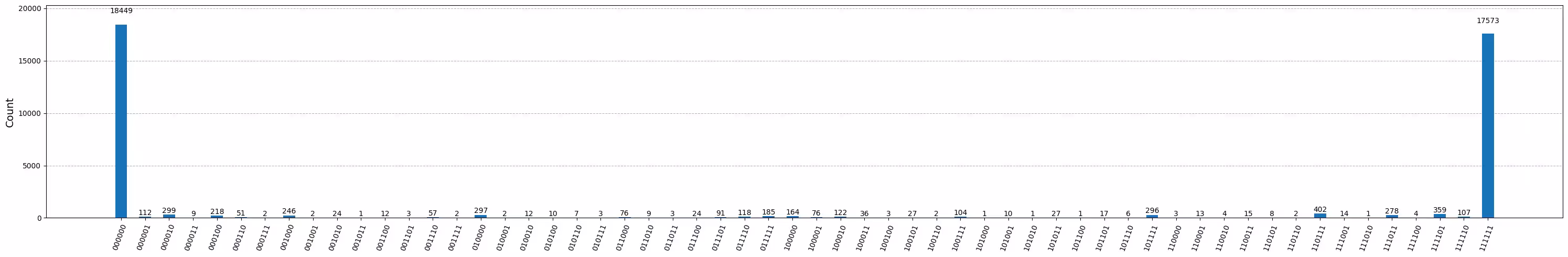
Questo è il risultato del circuito GHZ a 6 qubit. Come puoi vedere, gli stati di tutti $|0\rangle$ e tutti $|1\rangle$ dominano, ma gli errori sono sostanziali. Proviamo a vedere quanto grande può diventare un circuito GHZ su un dispositivo Eagle mantenendo comunque risultati in cui gli stati corretti abbiano probabilità di almeno il 50%.

1.2 Il tuo obiettivo

Costruisci un circuito GHZ per 20 qubit o più in modo che, alla misurazione, la fedeltà del tuo stato GHZ sia > 0,5. Nota:

• Devi usare un dispositivo Eagle (min_num_qubits=127) e impostare il numero di shots a 40.000.
• Devi eseguire il circuito GHZ usando la funzione execute_ghz_fidelity e calcolare la fedeltà usando la funzione check_ghz_fidelity_from_jobs.

Questo è pensato come un esercizio indipendente, in cui sfruttare ciò che hai imparato finora in questo corso.

def execute_ghz_fidelity(
    ghz_circuit: QuantumCircuit,  # Quantum circuit to create GHZ state (Circuit after Routing or without Routing), Classical register name is "c"
    physical_qubits: list[int],  # Physical qubits to represent GHZ state
    backend: BackendV2,
    sampler_options: dict | SamplerOptions | None = None,
):
    N_SHOTS = 40_000
    N = len(physical_qubits)
    base_circuit = ghz_circuit.remove_final_measurements(inplace=False)
    # M_k measurement circuits
    mk_circuits = []
    for k in range(1, N + 1):
        circuit = base_circuit.copy()
        # change measurement basis
        for q in physical_qubits:
            circuit.rz(-k * np.pi / N, q)
            circuit.h(q)
        mk_circuits.append(circuit)

    obs = SparsePauliOp.from_sparse_list(
        [("Z" * N, physical_qubits, 1)], num_qubits=backend.num_qubits
    )
    job_ids = []
    pm1 = generate_preset_pass_manager(1, backend=backend)
    org_transpiled = pm1.run(ghz_circuit)
    mk_transpiled = pm1.run(mk_circuits)
    with Batch(backend=backend):
        sampler = Sampler(options=sampler_options)
        sampler.options.twirling.enable_measure = True
        job = sampler.run([org_transpiled], shots=N_SHOTS)
        job_ids.append(job.job_id())
        # print(f"Sampler job id: {job.job_id()}, shots={N_SHOTS}")
        estimator = Estimator()  # TREX is applied as default
        estimator.options.dynamical_decoupling.enable = True
        estimator.options.execution.rep_delay = 0.0005
        estimator.options.twirling.enable_measure = True
        job2 = estimator.run([(circ, obs) for circ in mk_transpiled], precision=1 / 100)
        job_ids.append(job2.job_id())
        # print("Estimator job id:", job2.job_id())
        return [job.job_id(), job2.job_id()]

def check_ghz_fidelity_from_jobs(
    sampler_job,
    estimator_job,
    num_qubits,
    shots=40_000,
):
    N = num_qubits
    sampler_result = sampler_job.result()
    counts = sampler_result[0].data.c.get_counts()
    all_zero = counts.get("0" * N, 0) / shots
    all_one = counts.get("1" * N, 0) / shots
    top3 = sorted(counts, key=counts.get, reverse=True)[:3]
    print(
        f"N={N}: |00..0>: {counts.get('0'*N, 0)}, |11..1>: {counts.get('1'*N, 0)}, |3rd>: {counts.get(top3[2], 0)} ({top3[2]})"
    )
    print(f"P(|00..0>)={all_zero}, P(|11..1>)={all_one}")

    estimator_result = estimator_job.result()
    non_diagonal = (1 / N) * sum(
        (-1) ** k * estimator_result[k - 1].data.evs for k in range(1, N + 1)
    )
    print(f"REM: Coherence (non-diagonal): {non_diagonal:.6f}")
    fidelity = 0.5 * (all_zero + all_one + non_diagonal)
    sigma = 0.5 * np.sqrt(
        (1 - all_zero - all_one) * (all_zero + all_one) / shots
        + sum(estimator_result[k].data.stds ** 2 for k in range(N)) / (N * N)
    )
    print(f"GHZ fidelity = {fidelity:.6f} ± {sigma:.6f}")
    if fidelity - 2 * sigma > 0.5:
        print("GME (genuinely multipartite entangled) test: Passed")
    else:
        print("GME (genuinely multipartite entangled) test: Failed")
    return {
        "fidelity": fidelity,
        "sigma": sigma,
        "shots": shots,
        "job_ids": [sampler_job.job_id(), estimator_job.job_id()],
    }

In questo notebook, applicheremo tre strategie per creare buoni stati GHZ usando 16 qubit e 30 qubit. Questi approcci si basano su strategie che già conosci dalle lezioni precedenti.

2. Strategia 1. Selezione dei qubit consapevole del rumore

Per prima cosa specifichiamo un backend. Poiché lavoreremo a lungo con le proprietà di un backend specifico, è buona idea sceglierne uno fisso anziché usare l'opzione least_busy.

backend = service.backend("ibm_strasbourg")  # eagle
twoq_gate = "ecr"
print(f"Device {backend.name} Loaded with {backend.num_qubits} qubits")
print(f"Two Qubit Gate: {twoq_gate}")

Device ibm_strasbourg Loaded with 127 qubits
Two Qubit Gate: ecr

Costruiremo un circuito che coinvolge molti gate a due qubit. Ha senso usare i qubit con gli errori più bassi nell'implementazione di quei gate a due qubit. Trovare la migliore "catena di qubit" basandosi sugli errori riportati per i gate a 2 qubit è un problema non banale. Possiamo però definire alcune funzioni per determinare i qubit migliori da usare.

coupling_map = backend.target.build_coupling_map(twoq_gate)
G = coupling_map.graph

def to_edges(path):  # create edges list from node paths
    edges = []
    prev_node = None
    for node in path:
        if prev_node is not None:
            if G.has_edge(prev_node, node):
                edges.append((prev_node, node))
            else:
                edges.append((node, prev_node))
        prev_node = node
    return edges

def path_fidelity(path, correct_by_duration: bool = True, readout_scale: float = None):
    """Compute an estimate of the total fidelity of 2-qubit gates on a path.
    If `correct_by_duration` is true, each gate fidelity is worsen by
    scale = max_duration / duration, that is, gate_fidelity^scale.
    If `readout_scale` > 0 is supplied, readout_fidelity^readout_scale
    for each qubit on the path is multiplied to the total fielity.
    The path is given in node indices form, for example, [0, 1, 2].
    An external function `to_edges` is used to obtain edge list, for example, [(0, 1), (1, 2)]."""
    path_edges = to_edges(path)
    max_duration = max(backend.target[twoq_gate][qs].duration for qs in path_edges)

    def gate_fidelity(qpair):
        duration = backend.target[twoq_gate][qpair].duration
        scale = max_duration / duration if correct_by_duration else 1.0
        # 1.25 = (d+1)/d with d = 4
        return max(0.25, 1 - (1.25 * backend.target[twoq_gate][qpair].error)) ** scale

    def readout_fidelity(qubit):
        return max(0.25, 1 - backend.target["measure"][(qubit,)].error)

    total_fidelity = np.prod(
        [gate_fidelity(qs) for qs in path_edges]
    )  # two qubits gate fidelity for each path
    if readout_scale:
        total_fidelity *= (
            np.prod([readout_fidelity(q) for q in path]) ** readout_scale
        )  # multiply readout fidelity
    return total_fidelity

def flatten(paths, cutoff=None):  # cutoff is for not making run time too large
    return [
        path
        for s, s_paths in paths.items()
        for t, st_paths in s_paths.items()
        for path in st_paths[:cutoff]
        if s < t
    ]

N = 16  # Number of qubits to use in the GHZ circuit
num_qubits_in_chain = N

Useremo le funzioni di cui sopra per trovare tutti i percorsi semplici di N qubit tra tutte le coppie di nodi nel grafo (riferimento: all_pairs_all_simple_paths).

Poi, usando la funzione path_fidelity creata in precedenza, troveremo la migliore catena di qubit con la fedeltà di percorso più alta.

from functools import partial

%%time
paths = rx.all_pairs_all_simple_paths(
    G.to_undirected(multigraph=False),
    min_depth=num_qubits_in_chain,
    cutoff=num_qubits_in_chain,
)
paths = flatten(paths, cutoff=25)  # If you have time, you could set a larger cutoff.
if not paths:
    raise Exception(
        f"No qubit chain with length={num_qubits_in_chain} exists in {backend.name}. Try smaller num_qubits_in_chain."
    )

print(f"Selecting the best from {len(paths)} candidate paths")

best_qubit_chain = max(
    paths, key=partial(path_fidelity, correct_by_duration=True, readout_scale=1.0)
)
assert len(best_qubit_chain) == num_qubits_in_chain
print(f"Predicted (best possible) process fidelity: {path_fidelity(best_qubit_chain)}")

Selecting the best from 6046 candidate paths
Predicted (best possible) process fidelity: 0.8929026784775056
CPU times: user 284 ms, sys: 10.9 ms, total: 295 ms
Wall time: 295 ms

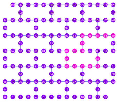
np.array(best_qubit_chain)

array([55, 49, 48, 47, 46, 45, 54, 64, 65, 66, 73, 85, 86, 87, 88, 89],
      dtype=uint64)

Visualizziamo la migliore catena di qubit, mostrata in rosa, nel diagramma della coupling map.

qubit_color = []
for i in range(133):
    if i in best_qubit_chain:
        qubit_color.append("#ff00dd")  # pink
    else:
        qubit_color.append("#8c00ff")  # purple
plot_gate_map(
    backend, qubit_color=qubit_color, qubit_size=50, font_size=25, figsize=(6, 6)
)

2.1 Costruire un circuito GHZ sulla migliore catena di qubit

Scegliamo un qubit al centro della catena a cui applicare per primo il gate H. Questo dovrebbe ridurre la profondità del circuito di circa la metà.

ghz1 = QuantumCircuit(max(best_qubit_chain) + 1, N)
ghz1.h(best_qubit_chain[N // 2])
for i in range(N // 2, 0, -1):
    ghz1.cx(best_qubit_chain[i], best_qubit_chain[i - 1])
for i in range(N // 2, N - 1, +1):
    ghz1.cx(best_qubit_chain[i], best_qubit_chain[i + 1])
ghz1.barrier()  # for visualization
ghz1.measure(best_qubit_chain, list(range(N)))
ghz1.draw(output="mpl", idle_wires=False, scale=0.5, fold=-1)

ghz1.depth()

10

pm = generate_preset_pass_manager(1, backend=backend)
ghz1_transpiled = pm.run(ghz1)
ghz1_transpiled.draw(output="mpl", idle_wires=False, fold=-1)

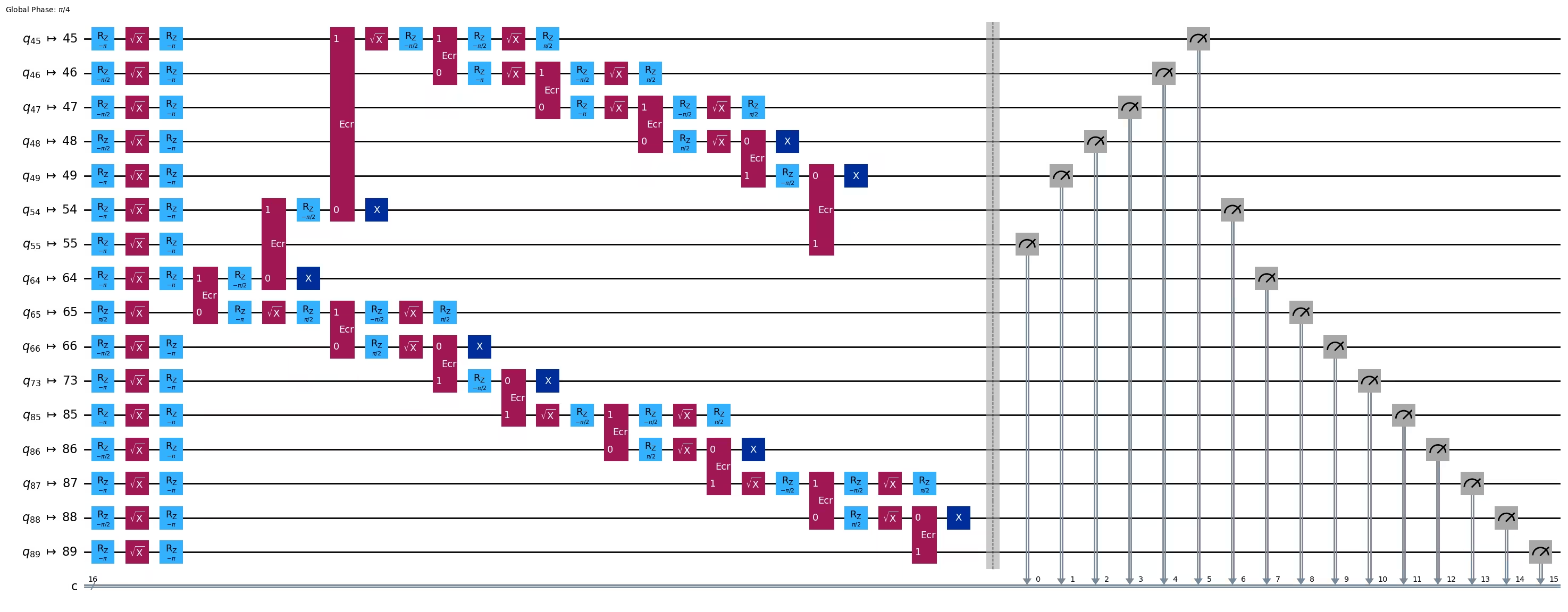
print("Depth:", ghz1_transpiled.depth())
print(
    "Two-qubit Depth:",
    ghz1_transpiled.depth(filter_function=lambda x: x.operation.num_qubits == 2),
)

Depth: 27
Two-qubit Depth: 8

opts = SamplerOptions()

res = execute_ghz_fidelity(
    ghz_circuit=ghz1,
    physical_qubits=best_qubit_chain,
    backend=backend,
    sampler_options=opts,
)

job_s = service.job(res[0])  # Use your job id showed above.
job_e = service.job(res[1])
print(job_s.status(), job_e.status())

DONE DONE

Fai attenzione ad eseguire la cella successiva solo dopo che gli stati dei job precedenti sono diventati 'DONE', per mostrare il risultato usando la funzione check_ghz_fidelity_from_jobs.

N = 16
# Check fidelity from job IDs
res = check_ghz_fidelity_from_jobs(
    sampler_job=job_s,
    estimator_job=job_e,
    num_qubits=N,
)

N=16: |00..0>: 153, |11..1>: 8681, |3rd>: 2262 (1111111111101111)
P(|00..0>)=0.003825, P(|11..1>)=0.217025
REM: Coherence (non-diagonal): 0.073809
GHZ fidelity = 0.147329 ± 0.002438
GME (genuinely multipartite entangled) test: Failed

result = job_s.result()
plot_histogram(result[0].data.c.get_counts(), figsize=(30, 5))

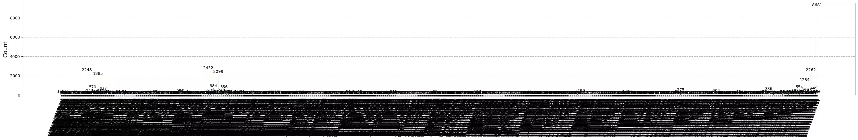
Questo risultato non soddisfa i criteri. Passiamo all'idea successiva.

3. Strategia 2. Albero bilanciato di qubit

L'idea successiva è trovare un albero bilanciato di qubit. Usando l'albero invece della catena, la profondità del circuito dovrebbe ridursi. Prima di procedere, rimuoviamo dal grafo di accoppiamento i nodi con errori di lettura "cattivi" e gli archi con errori di gate "cattivi".

BAD_READOUT_ERROR_THRESHOLD = 0.1
BAD_ECRGATE_ERROR_THRESHOLD = 0.1
bad_readout_qubits = [
    q
    for q in range(backend.num_qubits)
    if backend.target["measure"][(q,)].error > BAD_READOUT_ERROR_THRESHOLD
]
bad_ecrgate_edges = [
    qpair
    for qpair in backend.target["ecr"]
    if backend.target["ecr"][qpair].error > BAD_ECRGATE_ERROR_THRESHOLD
]
print("Bad readout qubits:", bad_readout_qubits)
print("Bad ECR gates:", bad_ecrgate_edges)

Bad readout qubits: [19, 28, 41, 72, 91, 114, 120]
Bad ECR gates: []

g = backend.coupling_map.graph.copy().to_undirected()
g.remove_edges_from(
    bad_ecrgate_edges
)  # remove edge first (otherwise might fail with a NoEdgeBetweenNodes error)
g.remove_nodes_from(bad_readout_qubits)

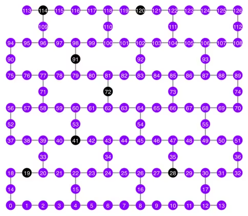
Disegniamo il grafo della mappa di accoppiamento senza gli archi e i qubit "cattivi".

qubit_color = []
for i in range(133):
    if i in bad_readout_qubits:
        qubit_color.append("#000000")  # black
    else:
        qubit_color.append("#8c00ff")  # purple
line_color = []
for e in backend.target.build_coupling_map().get_edges():
    if e in bad_ecrgate_edges:
        line_color.append("#ffffff")  # white
    else:
        line_color.append("#888888")  # gray
plot_gate_map(
    backend,
    qubit_color=qubit_color,
    line_color=line_color,
    qubit_size=50,
    font_size=25,
    figsize=(6, 6),
)

Proviamo a creare uno stato GHZ a 16 qubit come prima.

N = 16

Chiamiamo la funzione betweenness_centrality per trovare un qubit per il nodo radice. Il nodo con il valore più alto di centralità di betweenness si trova al centro del grafo. Riferimento: https://www.rustworkx.org/tutorial/betweenness_centrality.html

In alternativa, puoi selezionarlo manualmente.

# central = 65 #Select the center node manually
c_degree = dict(rx.betweenness_centrality(g))
central = max(c_degree, key=c_degree.get)
central

66

Partendo dal nodo radice, generiamo un albero tramite ricerca in ampiezza (BFS). Riferimento: https://qiskit.org/ecosystem/rustworkx/apiref/rustworkx.bfs_search.html#rustworkx-bfs-search

class TreeEdgesRecorder(rx.visit.BFSVisitor):
    def __init__(self, N):
        self.edges = []
        self.N = N

    def tree_edge(self, edge):
        self.edges.append(edge)
        if len(self.edges) >= self.N - 1:
            raise rx.visit.StopSearch()

vis = TreeEdgesRecorder(N)
rx.bfs_search(g, [central], vis)
best_qubits = sorted(list(set(q for e in vis.edges for q in (e[0], e[1]))))
# print('Tree edges:', vis.edges)

print("Qubits selected:", best_qubits)

Qubits selected: [54, 55, 63, 64, 65, 66, 67, 68, 69, 70, 73, 83, 84, 85, 86, 87]

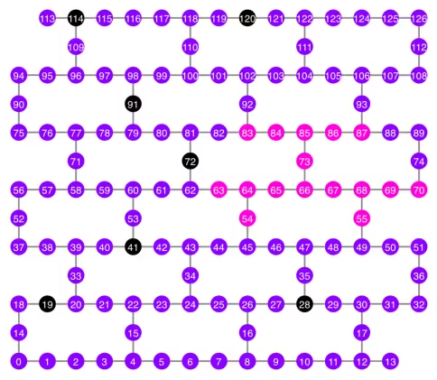
Tracciamo i qubit selezionati, mostrati in rosa, nel diagramma della mappa di accoppiamento.

qubit_color = []
for i in range(133):
    if i in bad_readout_qubits:
        qubit_color.append("#000000")  # black
    elif i in best_qubits:
        qubit_color.append("#ff00dd")  # pink
    else:
        qubit_color.append("#8c00ff")  # purple
plot_gate_map(
    backend,
    qubit_color=qubit_color,
    line_color=line_color,
    qubit_size=50,
    font_size=25,
    figsize=(6, 6),
)

Mostriamo la struttura ad albero dei qubit.

from rustworkx.visualization import graphviz_draw

tree = rx.PyDiGraph()
tree.extend_from_weighted_edge_list(vis.edges)
tree.remove_nodes_from([n for n in range(max(best_qubits) + 1) if n not in best_qubits])

graphviz_draw(tree, method="dot")

ghz2 = QuantumCircuit(max(best_qubits) + 1, N)

ghz2.h(tree.edge_list()[0][0])  # apply H-gate to the root node
# Apply CNOT from the root node to the each edge.
for u, v in tree.edge_list():
    ghz2.cx(u, v)
ghz2.barrier()  # for visualization
ghz2.measure(best_qubits, list(range(N)))
ghz2.draw(output="mpl", idle_wires=False, scale=0.5)

ghz2.depth()

8

pm = generate_preset_pass_manager(1, backend=backend)
ghz2_transpiled = pm.run(ghz2)
ghz2_transpiled.draw(output="mpl", idle_wires=False, fold=-1)

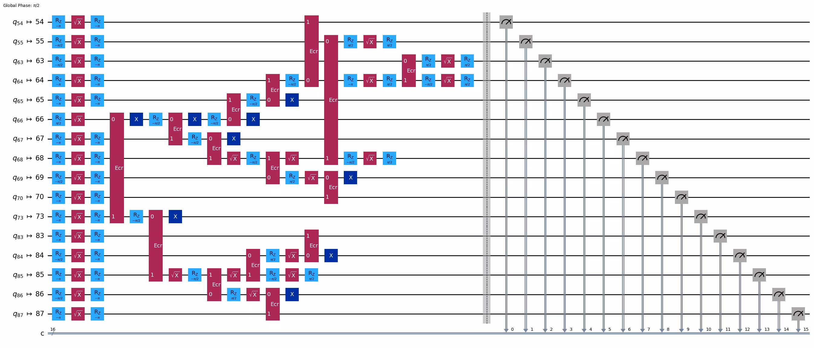
print("Depth:", ghz2_transpiled.depth())
print(
    "Two-qubit Depth:",
    ghz2_transpiled.depth(filter_function=lambda x: x.operation.num_qubits == 2),
)

Depth: 22
Two-qubit Depth: 6

La profondità del circuito è ora diventata molto inferiore rispetto alla struttura a catena.

res = execute_ghz_fidelity(
    ghz_circuit=ghz2,
    physical_qubits=best_qubits,
    backend=backend,
    sampler_options=opts,
)

job_s = service.job(res[0])  # Use your job id showed above.
job_e = service.job(res[1])
print(job_s.status(), job_e.status())

DONE DONE

N = 16
# Check fidelity from job IDs
res = check_ghz_fidelity_from_jobs(
    sampler_job=job_s,
    estimator_job=job_e,
    num_qubits=N,
)

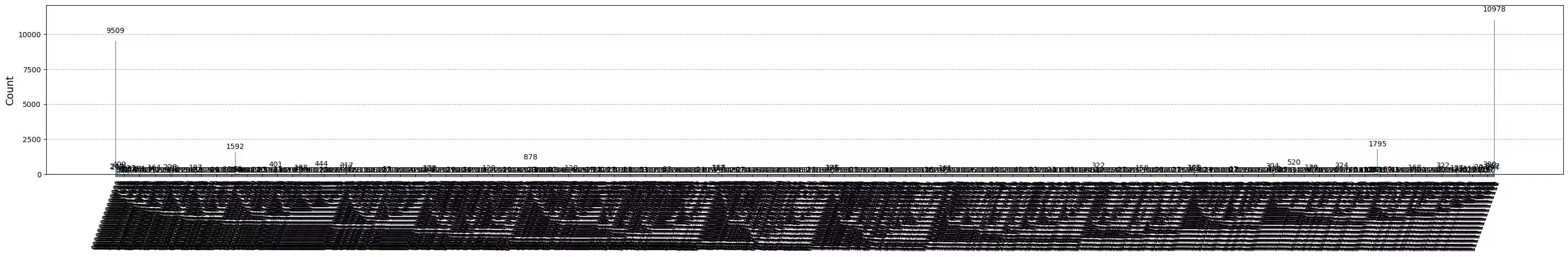
N=16: |00..0>: 9509, |11..1>: 10978, |3rd>: 1795 (1111110111111111)
P(|00..0>)=0.237725, P(|11..1>)=0.27445
REM: Coherence (non-diagonal): 0.606515
GHZ fidelity = 0.559345 ± 0.003188
GME (genuinely multipartite entangled) test: Passed

Abbiamo superato con successo i criteri con la struttura ad albero bilanciato!

result = job_s.result()
plot_histogram(result[0].data.c.get_counts(), figsize=(30, 5))

Ora proviamo a creare uno stato GHZ più grande: uno stato GHZ a 30 qubit.

3.1 N = 30

Seguiremo il framework dei pattern Qiskit.

• Passo 1: Mappare il problema in circuiti quantistici e operatori
• Passo 2: Ottimizzare per l'hardware target
• Passo 3: Eseguire sull'hardware target
• Passo 4: Post-elaborare i risultati

Passo 1: Mappare il problema in circuiti quantistici e operatori e Passo 2: Ottimizzare per l'hardware target

Qui selezioniamo manualmente il nodo radice.

central = 62  # Select the center node manually
# c_degree = dict(rx.betweenness_centrality(g))
# central = max(c_degree, key=c_degree.get)
# central

N = 30

vis = TreeEdgesRecorder(N)
rx.bfs_search(g, [central], vis)
best_qubits = sorted(list(set(q for e in vis.edges for q in (e[0], e[1]))))
print("Qubits selected:", best_qubits)

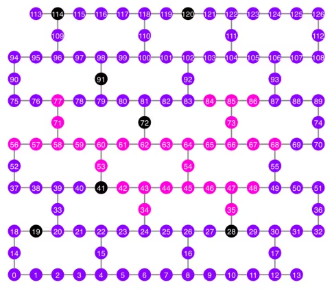
Qubits selected: [34, 35, 42, 43, 44, 45, 46, 47, 48, 53, 54, 56, 57, 58, 59, 60, 61, 62, 63, 64, 65, 66, 67, 68, 71, 73, 77, 84, 85, 86]

qubit_color = []
for i in range(133):
    if i in bad_readout_qubits:
        qubit_color.append("#000000")
    elif i in best_qubits:
        qubit_color.append("#ff00dd")
    else:
        qubit_color.append("#8c00ff")
line_color = []
for e in backend.target.build_coupling_map().get_edges():
    if e in bad_ecrgate_edges:
        line_color.append("#ffffff")
    else:
        line_color.append("#888888")
plot_gate_map(
    backend,
    qubit_color=qubit_color,
    line_color=line_color,
    qubit_size=50,
    font_size=25,
    figsize=(6, 6),
)

from rustworkx.visualization import graphviz_draw

tree = rx.PyDiGraph()
tree.extend_from_weighted_edge_list(vis.edges)
tree.remove_nodes_from([n for n in range(max(best_qubits) + 1) if n not in best_qubits])

graphviz_draw(tree, method="dot")

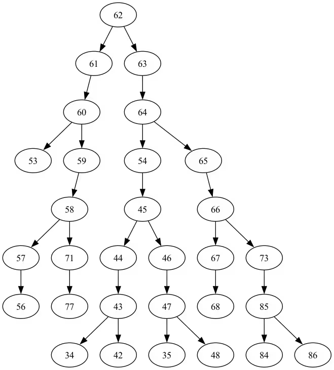
La profondità di quest'albero è 5.

ghz3 = QuantumCircuit(max(best_qubits) + 1, N)

ghz3.h(tree.edge_list()[0][0])  # apply H-gate to the root node
# Apply CNOT from the root node to the each edge.
for u, v in tree.edge_list():
    ghz3.cx(u, v)
ghz3.barrier()  # for visualization
ghz3.measure(best_qubits, list(range(N)))
ghz3.draw(output="mpl", idle_wires=False, fold=-1)

ghz3.depth()

11

pm = generate_preset_pass_manager(1, backend=backend)
ghz3_transpiled = pm.run(ghz3)
ghz3_transpiled.draw(output="mpl", idle_wires=False, fold=-1)

print("Depth:", ghz3_transpiled.depth())
print(
    "Two-qubit Depth:",
    ghz3_transpiled.depth(filter_function=lambda x: x.operation.num_qubits == 2),
)

Depth: 31
Two-qubit Depth: 9

3.2 Seleziona manualmente un nodo radice diverso

central = 54

vis = TreeEdgesRecorder(N)
rx.bfs_search(g, [central], vis)
best_qubits = sorted(list(set(q for e in vis.edges for q in (e[0], e[1]))))
print("Qubits selected:", best_qubits)

Qubits selected: [23, 24, 25, 34, 35, 42, 43, 44, 45, 46, 47, 48, 49, 50, 54, 55, 60, 61, 62, 63, 64, 65, 66, 67, 68, 69, 73, 84, 85, 86]

from rustworkx.visualization import graphviz_draw

tree = rx.PyDiGraph()
tree.extend_from_weighted_edge_list(vis.edges)
tree.remove_nodes_from([n for n in range(max(best_qubits) + 1) if n not in best_qubits])

graphviz_draw(tree, method="dot")

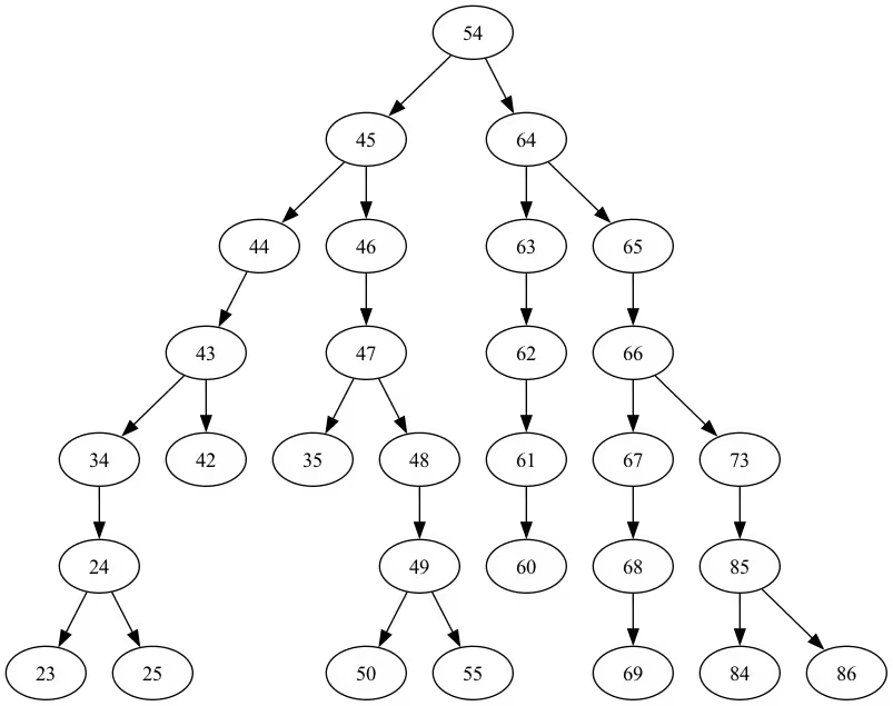
La profondità di quest'albero è 6.

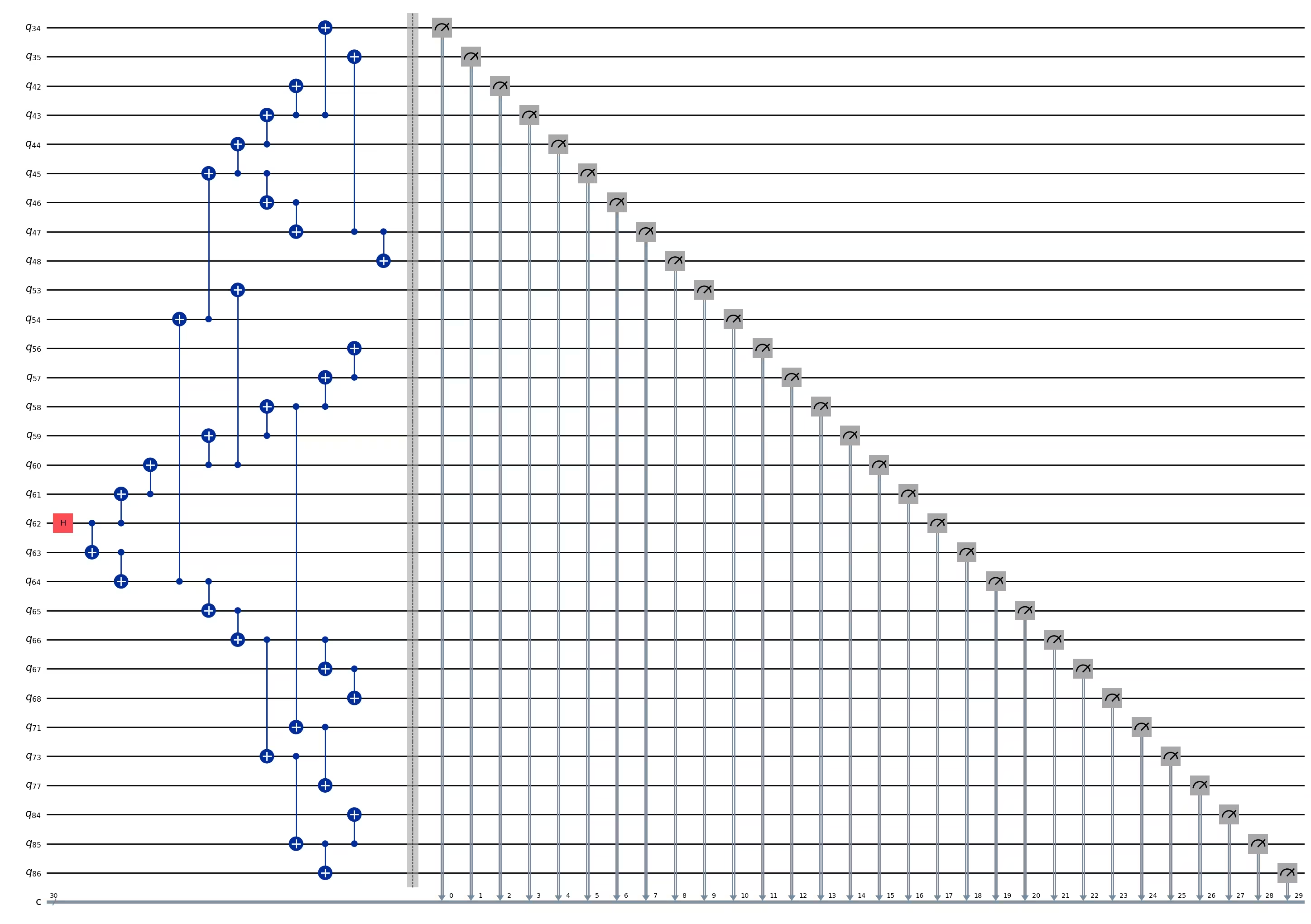
ghz3 = QuantumCircuit(max(best_qubits) + 1, N)

ghz3.h(tree.edge_list()[0][0])  # apply H-gate to the root node
# Apply CNOT from the root node to the each edge.
for u, v in tree.edge_list():
    ghz3.cx(u, v)
ghz3.barrier()  # for visualization
ghz3.measure(best_qubits, list(range(N)))
ghz3.draw(output="mpl", idle_wires=False, fold=-1)

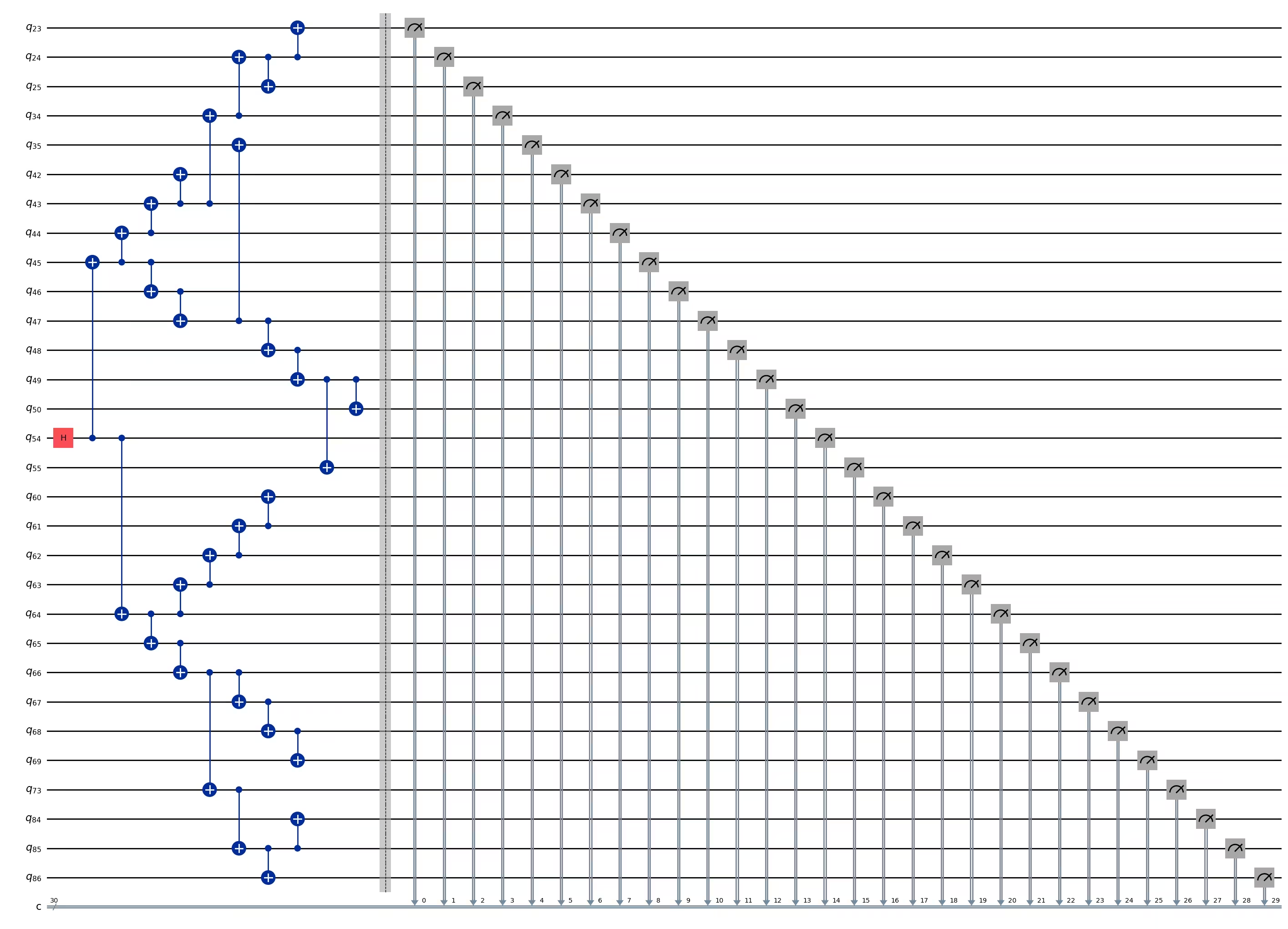
ghz3.depth()

11

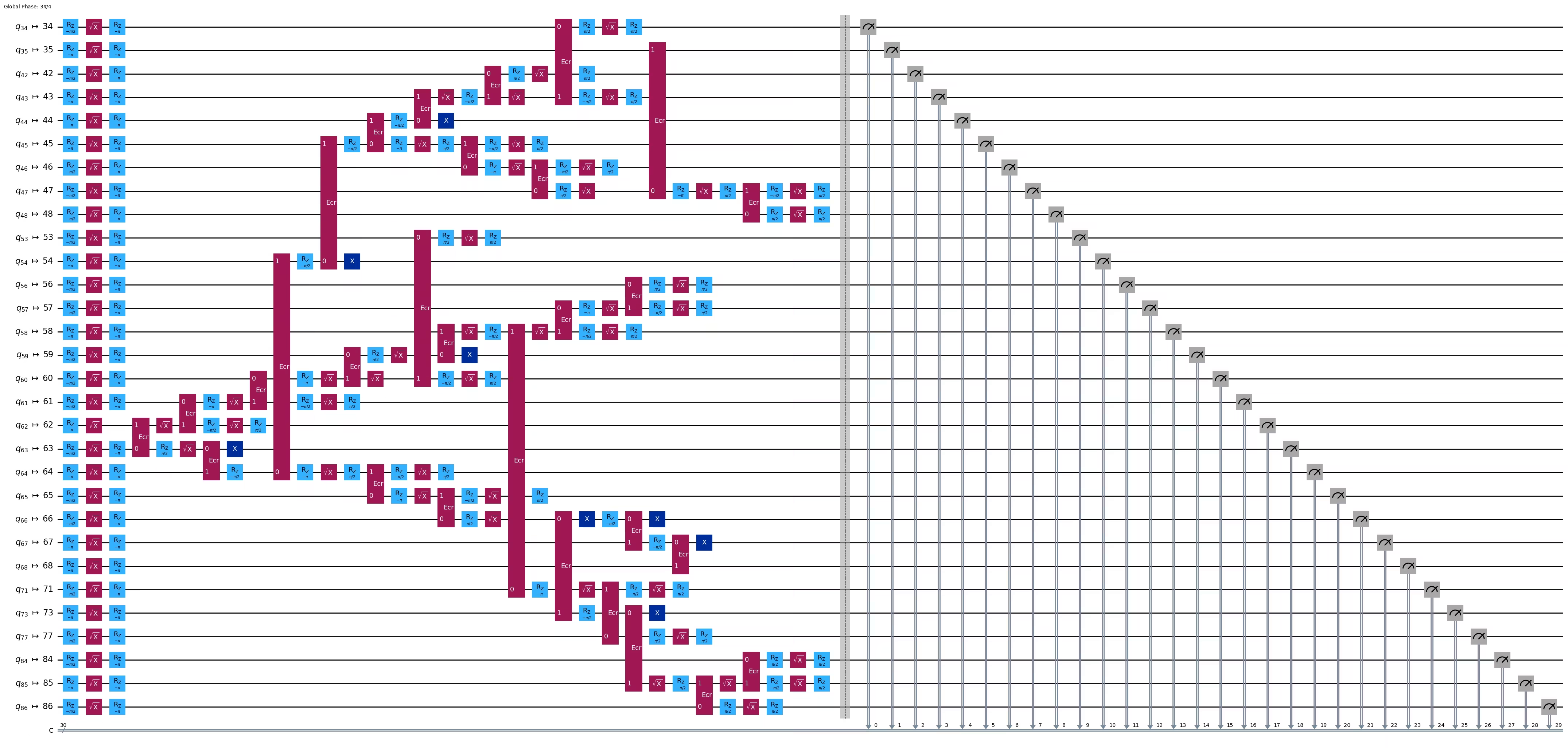
pm = generate_preset_pass_manager(1, backend=backend)
ghz3_transpiled = pm.run(ghz3)
ghz3_transpiled.draw(output="mpl", idle_wires=False, fold=-1)

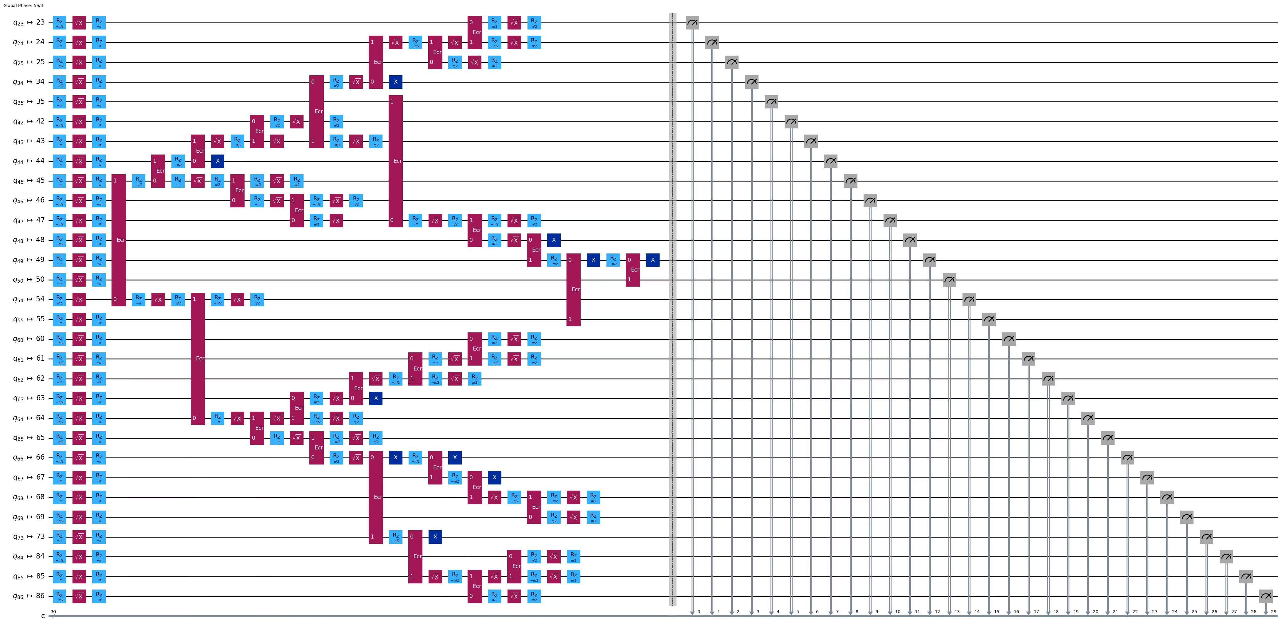
print("Depth:", ghz3_transpiled.depth())
print(
    "Two-qubit Depth:",
    ghz3_transpiled.depth(filter_function=lambda x: x.operation.num_qubits == 2),
)

Depth: 30
Two-qubit Depth: 9

Sorprendentemente, mentre la profondità dell'albero è aumentata da 5 a 6, la profondità a due qubit è diminuita da 9 a 8! Usiamo quindi quest'ultimo circuito.

Passo 3: Eseguire sull'hardware target

res = execute_ghz_fidelity(
    ghz_circuit=ghz3,
    physical_qubits=best_qubits,
    backend=backend,
    sampler_options=opts,
)

job_s = service.job(res[0])  # Use your job id showed above.
job_e = service.job(res[1])
print(job_s.status(), job_e.status())

DONE DONE

Passo 4: Post-elaborare i risultati

N = 30
# Check fidelity from job IDs
res = check_ghz_fidelity_from_jobs(
    sampler_job=job_s,
    estimator_job=job_e,
    num_qubits=N,
)

N=30: |00..0>: 4, |11..1>: 218, |3rd>: 265 (111111111111111011111111111111)
P(|00..0>)=0.0001, P(|11..1>)=0.00545
REM: Coherence (non-diagonal): 0.187073
GHZ fidelity = 0.096312 ± 0.003254
GME (genuinely multipartite entangled) test: Failed

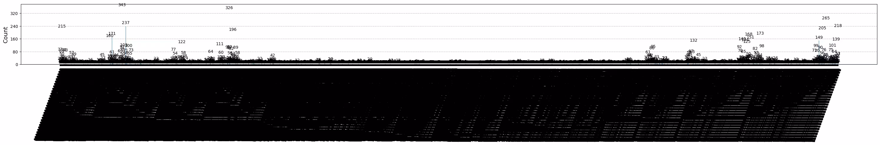
Come puoi vedere, questo risultato non soddisfa i criteri.

# It will take some time
result = job_s.result()
plot_histogram(result[0].data.c.get_counts(), figsize=(30, 5))

4. Strategia 3. Eseguire con le opzioni di soppressione degli errori

Puoi impostare le opzioni di soppressione degli errori in Sampler V2. Consulta la guida Configurare la mitigazione degli errori e il riferimento API ExecutionOptionsV2 per ulteriori informazioni.

opts = SamplerOptions()
opts.dynamical_decoupling.enable = True
opts.execution.rep_delay = 0.0005
opts.twirling.enable_gates = True

res = execute_ghz_fidelity(
    ghz_circuit=ghz3,
    physical_qubits=best_qubits,
    backend=backend,
    sampler_options=opts,
)

job_s = service.job(res[0])  # Use your job id showed above.
job_e = service.job(res[1])
print(job_s.status(), job_e.status())

DONE DONE

N = 30

# Check fidelity from job IDs
res = check_ghz_fidelity_from_jobs(
    sampler_job=job_s,
    estimator_job=job_e,
    num_qubits=N,
)

N=30: |00..0>: 1459, |11..1>: 1543, |3rd>: 359 (111111111111111111111111111110)
P(|00..0>)=0.036475, P(|11..1>)=0.038575
REM: Coherence (non-diagonal): 0.165532
GHZ fidelity = 0.120291 ± 0.003369
GME (genuinely multipartite entangled) test: Failed

# It will take some time
result = job_s.result()
plot_histogram(result[0].data.c.get_counts(), figsize=(30, 5))

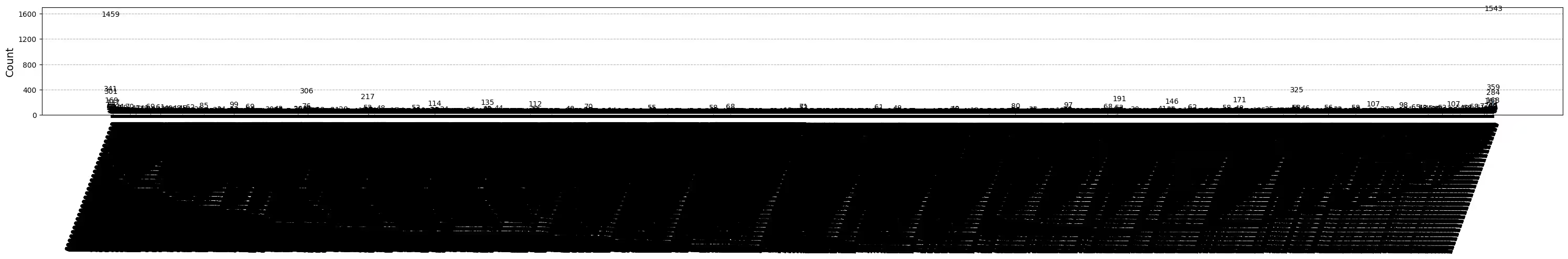
Il risultato è migliorato ma non soddisfa ancora i criteri.

Abbiamo visto tre idee finora. Puoi combinarle e ampliarle oppure sviluppare le tue idee per creare un circuito GHZ migliore. Ora rivediamo l'obiettivo.

5. Il tuo obiettivo (riepilogo)

Costruisci un circuito GHZ per 20 qubit o più in modo che il risultato della misurazione soddisfi i criteri: la fedeltà del tuo stato GHZ > 0,5.

• Devi usare un dispositivo Eagle (come ibm_brisbane) e impostare il numero di shots a 40.000.
• Devi eseguire il circuito GHZ usando la funzione execute_ghz_fidelity e calcolare la fedeltà con la funzione check_ghz_fidelity_from_jobs. Devi trovare il circuito GHZ con il maggior numero di qubit che soddisfi i criteri. Scrivi il tuo codice qui sotto e mostra il risultato con la funzione check_ghz_fidelity_from_jobs.

Ora implementiamo lo stesso flusso di lavoro GHZ del materiale precedente, ma su un dispositivo Heron. Questo ti dà un po' di esperienza con il layout e le caratteristiche dei processori Heron. Non vengono introdotte nuove strategie.

Il tempo QPU approssimativo per eseguire questo esperimento è di 4 min 40 s.

service = QiskitRuntimeService()
backend = service.backend("ibm_kingston")
# backend = service.backend("ibm_fez")

twoq_gate = "cz"
print(f"Device {backend.name} Loaded with {backend.num_qubits} qubits")
print(f"Two Qubit Gate: {twoq_gate}")

Device ibm_kingston Loaded with 156 qubits
Two Qubit Gate: cz

BAD_READOUT_ERROR_THRESHOLD = 0.1
BAD_CZGATE_ERROR_THRESHOLD = 0.1
bad_readout_qubits = [
    q
    for q in range(backend.num_qubits)
    if backend.target["measure"][(q,)].error > BAD_READOUT_ERROR_THRESHOLD
]
bad_czgate_edges = [
    qpair
    for qpair in backend.target["cz"]
    if backend.target["cz"][qpair].error > BAD_CZGATE_ERROR_THRESHOLD
]
print("Bad readout qubits:", bad_readout_qubits)
print("Bad CZ gates:", bad_czgate_edges)

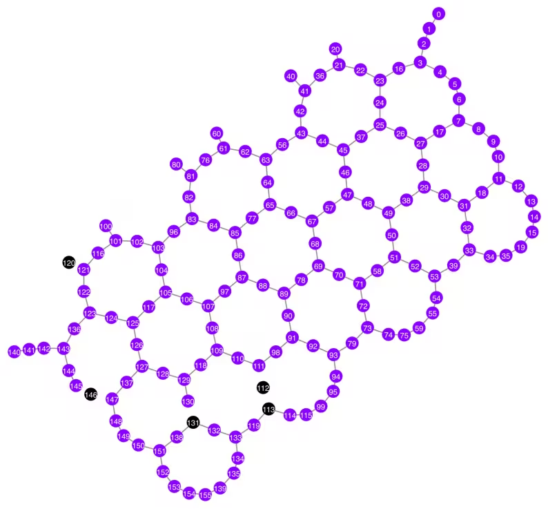
Bad readout qubits: [112, 113, 120, 131, 146]
Bad CZ gates: [(111, 112), (112, 111), (112, 113), (113, 112), (120, 121), (121, 120), (130, 131), (131, 130), (145, 146), (146, 145), (146, 147), (147, 146)]

g = backend.coupling_map.graph.copy().to_undirected()
g.remove_edges_from(
    bad_czgate_edges
)  # remove edge first (otherwise might fail with a NoEdgeBetweenNodes error)
g.remove_nodes_from(bad_readout_qubits)

qubit_color = []
for i in range(backend.num_qubits):
    if i in bad_readout_qubits:
        qubit_color.append("#000000")  # black
    else:
        qubit_color.append("#8c00ff")  # purple
line_color = []
for e in backend.target.build_coupling_map().get_edges():
    if e in bad_czgate_edges:
        line_color.append("#ffffff")  # white
    else:
        line_color.append("#888888")  # gray
plot_gate_map(
    backend,
    qubit_color=qubit_color,
    line_color=line_color,
    qubit_size=60,
    font_size=30,
    figsize=(10, 10),
)

N = 40
central = 100  # Select the center node manually
# c_degree = dict(rx.betweenness_centrality(g))
# central = max(c_degree, key=c_degree.get)
# central

class TreeEdgesRecorder(rx.visit.BFSVisitor):
    def __init__(self, N):
        self.edges = []
        self.N = N

    def tree_edge(self, edge):
        self.edges.append(edge)
        if len(self.edges) >= self.N - 1:
            raise rx.visit.StopSearch()

vis = TreeEdgesRecorder(N)
rx.bfs_search(g, [central], vis)
best_qubits = sorted(list(set(q for e in vis.edges for q in (e[0], e[1]))))
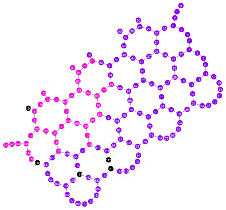
print("Qubits selected:", best_qubits)

Qubits selected: [61, 65, 76, 77, 80, 81, 82, 83, 84, 85, 86, 87, 96, 97, 100, 101, 102, 103, 104, 105, 106, 107, 108, 109, 116, 117, 121, 122, 123, 124, 125, 126, 127, 136, 140, 141, 142, 143, 144, 145]

qubit_color = []
for i in range(backend.num_qubits):
    if i in bad_readout_qubits:
        qubit_color.append("#000000")
    elif i in best_qubits:
        qubit_color.append("#ff00dd")
    else:
        qubit_color.append("#8c00ff")
line_color = []
for e in backend.target.build_coupling_map().get_edges():
    if e in bad_czgate_edges:
        line_color.append("#ffffff")
    else:
        line_color.append("#888888")
plot_gate_map(
    backend,
    qubit_color=qubit_color,
    line_color=line_color,
    qubit_size=60,
    font_size=30,
    figsize=(10, 10),
)

from rustworkx.visualization import graphviz_draw

tree = rx.PyDiGraph()
tree.extend_from_weighted_edge_list(vis.edges)
tree.remove_nodes_from([n for n in range(max(best_qubits) + 1) if n not in best_qubits])

graphviz_draw(tree, method="dot")

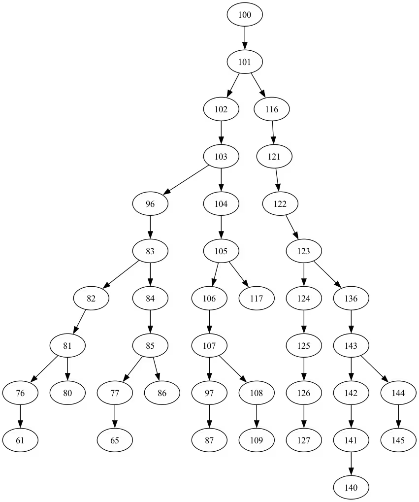
ghz_h = QuantumCircuit(max(best_qubits) + 1, N)

ghz_h.h(tree.edge_list()[0][0])  # apply H-gate to the root node
# Apply CNOT from the root node to the each edge.
for u, v in tree.edge_list():
    ghz_h.cx(u, v)
ghz_h.barrier()  # for visualization
ghz_h.measure(best_qubits, list(range(N)))
ghz_h.draw(output="mpl", idle_wires=False, fold=-1)

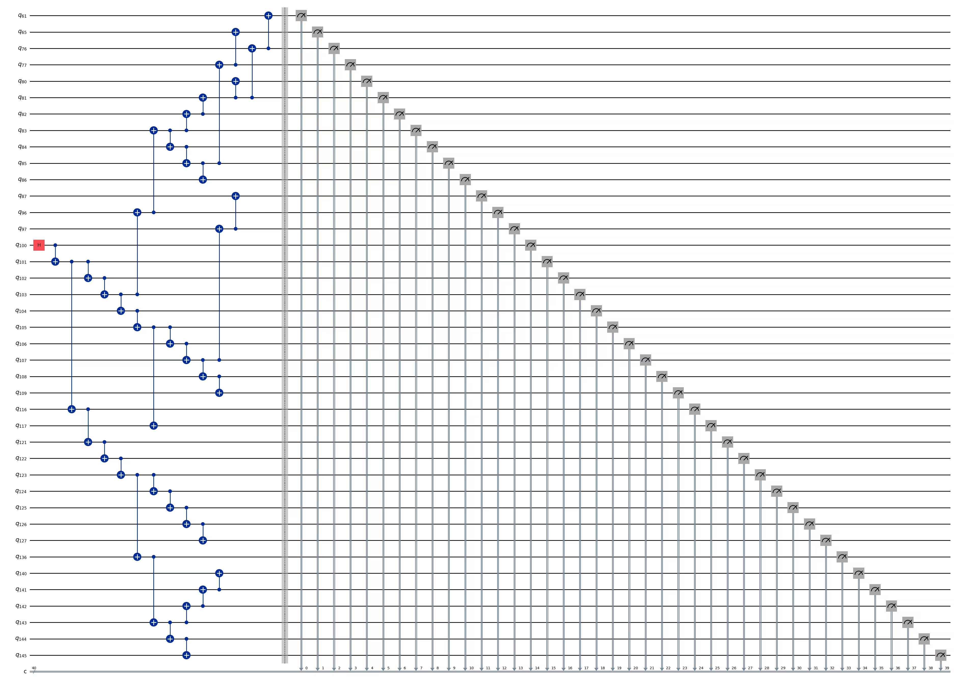
ghz_h.depth()

15

pm = generate_preset_pass_manager(1, backend=backend)
ghz_h_transpiled = pm.run(ghz_h)
ghz_h_transpiled.draw(output="mpl", idle_wires=False, fold=-1)

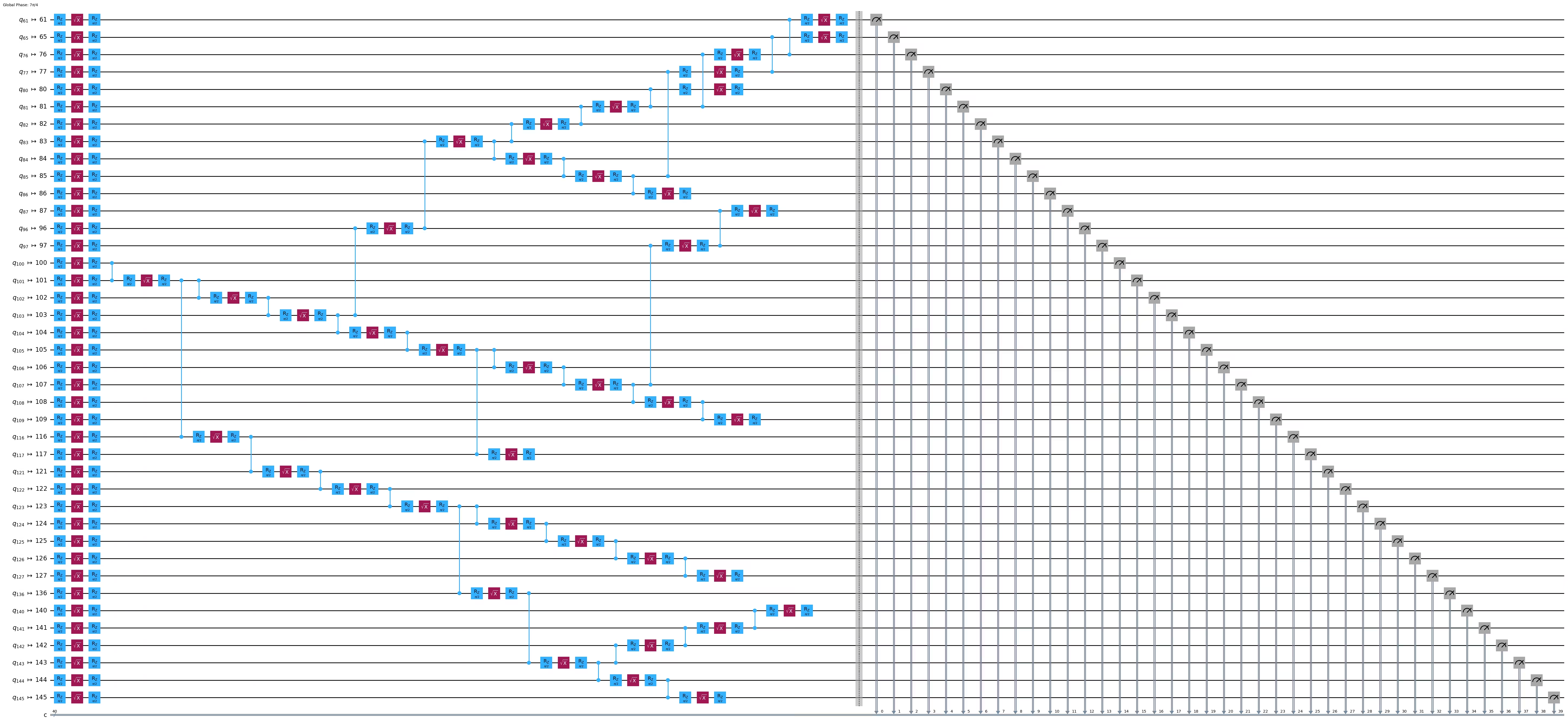
print("Depth:", ghz_h_transpiled.depth())
print(
    "Two-qubit Depth:",
    ghz_h_transpiled.depth(filter_function=lambda x: x.operation.num_qubits == 2),
)

Depth: 45
Two-qubit Depth: 13

opts = SamplerOptions()
opts.dynamical_decoupling.enable = True
opts.execution.rep_delay = 0.0005
opts.twirling.enable_gates = True

res = execute_ghz_fidelity(
    ghz_circuit=ghz_h,
    physical_qubits=best_qubits,
    backend=backend,
    sampler_options=opts,
)

job_s = service.job(res[0])  # Use your job id showed above.
job_e = service.job(res[1])
print(job_s.status(), job_e.status())

RUNNING RUNNING

# Check fidelity from job IDs
N = 40
res = check_ghz_fidelity_from_jobs(
    sampler_job=job_s,
    estimator_job=job_e,
    num_qubits=N,
)

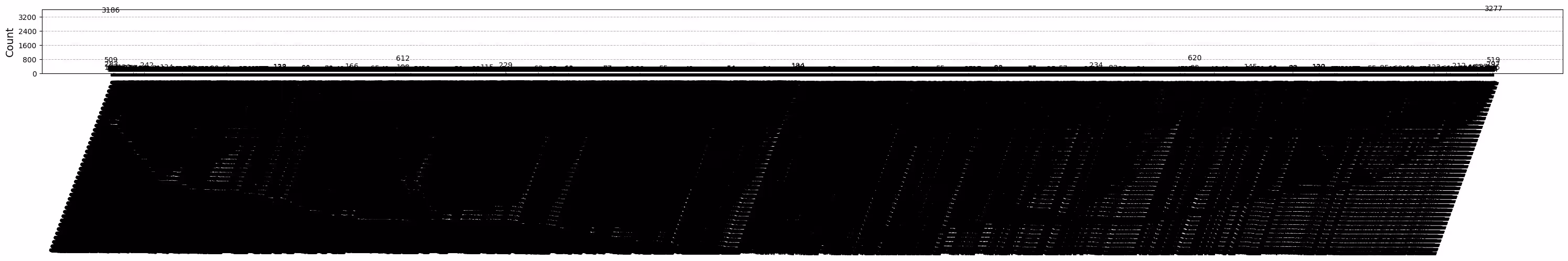
N=40: |00..0>: 3186, |11..1>: 3277, |3rd>: 620 (1111111011111111111111111111111111111111)
P(|00..0>)=0.07965, P(|11..1>)=0.081925
REM: Coherence (non-diagonal): 0.029987
GHZ fidelity = 0.095781 ± 0.002619
GME (genuinely multipartite entangled) test: Failed

# It will take some time
result = job_s.result()
plot_histogram(result[0].data.c.get_counts(), figsize=(30, 5))

Congratulazioni! Hai completato la tua introduzione al calcolo quantistico su scala di utilità! Sei ora pronto a dare contributi significativi nella ricerca del vantaggio quantistico! Grazie per aver fatto di IBM Quantum® parte del tuo percorso personale nel mondo della quantistica.

Sondaggio post-corso

Congratulazioni per aver completato questo corso! Prenditi un momento per aiutarci a migliorare il nostro corso compilando il seguente breve sondaggio. Il tuo feedback verrà utilizzato per migliorare i nostri contenuti e l'esperienza utente. Grazie!